
NUMERICAL STABILITY; IMPLICIT METHODS
If a numerical method has no restrictions on in order to have y n!0 as n !1, we say the numerical method is A-stable. THE BACKWARD EULER METHOD Expand the function Y(x) as a linear Taylor polynomial about x n+1: Y(x) = Y(x n+1) + (x x n+1)Y0(x n+1) + 1 2 (x x n+1) 2 Y00( n) with n between x and x n+1. Let x = x
Download NUMERICAL STABILITY; IMPLICIT METHODS

Information
Domain:
Source:
Link to this page:
Documents from same domain

THE SECANT METHOD - University of Iowa
homepage.math.uiowa.eduTHE SECANT METHOD Newton’s method was based on using the line tangent to the curve of y = f(x), with the point of tangency (x 0;f(x 0)).When x 0 ˇ , the graph of the tangent line is approximately the same as the

NUMERICALSOLUTIONOF ORDINARYDIFFERENTIAL …
homepage.math.uiowa.eduThe differential equations we consider in most of the book are of the form Y′(t) = f(t,Y(t)), where Y(t) is an unknown function that is being sought. The given function f(t,y) of two variables defines the differential equation, and exam ples are given in Chapter 1. This equation is called a first-order differential equation because it ...

Lecture 1: The Euler characteristic
homepage.math.uiowa.edu7 vertices, 9 edges, 2 faces. We wish to count: 3 vertices, 3 edges, 1 face. 6 vertices, 9 edges, 4 faces. Euler characteristic (simple form): = number of vertices – number of edges + number of faces Or in short-hand, = |V| - |E| + |F| where V = set of vertices E = set of edges ...
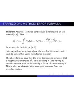
TRAPEZOIDAL METHOD: ERROR FORMULA
homepage.math.uiowa.eduThe corrected trapezoidal rule is illustrated in the following table. n I T n Ratio I CT n Ratio 2 5.319 3.552E 1 4 1.266 4.20 2.474E 2 14.4 8 3.118E 1 4.06 1.583E 3 15.6

ERROR IN LINEAR INTERPOLATION
homepage.math.uiowa.eduFor f(x) = log 10 x, with 1 x 0 x x 2 10; this leads to jlog 10 x P 2(x)j h3 9 p 3 max x0 x x2 2log 10 e x3:05572h3 x3 0 For the case of h = :01, we have jlog 10 x P 2(x)j 5:57 10 8 x3 0 5:57 10 8 For comparison, jlog 10 x P 1(x)j 5:43 10 6
A quick example calculating the column space and the ...
homepage.math.uiowa.eduPut A into echelon form and then into reduced echelon form: R 2 –R 1 R 2 R 3 + 2R 1 R 3 R 1 + 5R 2 R 1 R 2 /2 R 2 R 1 + 8R 3 ...
Related documents

Chapter 5: Numerical Integration and Differentiation
www.ece.mcmaster.caChapter 5: Numerical Integration and Differentiation PART I: Numerical Integration Newton-Cotes Integration Formulas The idea of Newton-Cotes formulas is to replace a complicated function or tabu-lated data with an approximating function that is easy to integrate. I = Z b a f(x)dx … Z b a fn(x)dx where fn(x) = a0 +a1x+a2x2 +:::+anxn. 1 The ...

Convergence of Numerical Methods
web.mit.eduChapter 2 Convergence of Numerical Methods In the last chapter we derived the forward Euler method from a Taylor series expansion of un+1 and we utilized the method on some simple example problems without any supporting analysis.
Chapter 10 Numerical solution methods - San Jose State ...
www.sjsu.eduNumerical methods are techniques by which the mathematical problems involved with the engineering analysis cannot readily or possibly be solved by analytical methods such as those presented in previous chapters of this book. We will learn from this chapter on the use of some of these numerical methods that will

1.10 Numerical Solution to First-Order Differential Equations
www.math.purdue.eduideas associated with constructing numerical solutions to initial-value problems that are beyond the scope of this text. Indeed, a full discussion of the application of numerical methods to differential equations is best left for a future course in numerical analysis. Euler’s Method
Applications of Numerical Methods in Engineering CNS 3320
www-personal.umich.eduNumerical Integration Example: Falling Climber T can be determined analytically, how the rope deflects requires numerical methods. T = V = Z δ f 0 F·dr The rope behaves as a nonlinear spring, and the force the rope exerts F is an unknown function of its deflection δ. • F(δ)determinedexperimentallywith discrete samples.
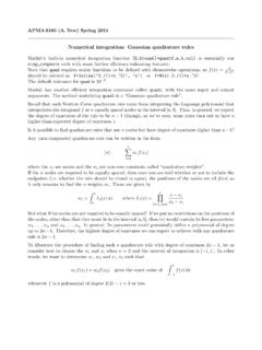
Numerical integration: Gaussian quadrature rules
www.dam.brown.eduNumerical integration: Gaussian quadrature rules Matlab’s built-in numerical integration function [Q,fcount]=quad(f,a,b,tol) is essentially our simp_compextr code with some further efficiency-enhancing features. Note that quad requires scalar functions to be defined with elementwise operations, so f(x) = 2 1+x2

Writing and Interpreting Numerical Expressions
members.mathteachercoach.comMar 01, 2016 · Writing and Interpreting Numerical Expressions Students will be able to: •Recognize numerical expressions. •Familiarize the words used to represent operations such as addition, subtraction, multiplication and division. •Write a numerical expression that record calculations with numbers given a verbal phrase.
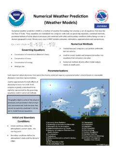
Numerical Weather Prediction (Weather Models)
www.weather.govNumerical weather prediction (NWP) is a method of weather forecasting that employs a set of equations that describe the flow of fluids. These equations are translated into computer code and use governing equations, numerical methods,

Numerical differentiation: finite differences
www.dam.brown.eduNumerical differentiation: finite differences The derivative of a function f at the point x is defined as the limit of a difference quotient: f0(x) = lim h→0 f(x+h)−f(x) h In other words, the difference quotient f(x+h)−f(x) h is an approximation of the derivative f0(x), and this approximation gets better as h gets smaller.