The Logit Model: Estimation, Testing and Interpretation

1 The Logit Model: estimation , Testing and InterpretationHerman J. BierensOctober 25, 20081 Introduction to maximum likelihood The likelihood functionConsider a random sampleY1, .., Ynfrom the Bernoulli distribution:Pr[Yj=1]=p0Pr[Yj=0]=1 p0,wherep0is unknown. For example, tossntimes a coin for which you suspectthat it is unfair:p06= ,and for each tossingjassignYj=1if the outcomeis heads andYj=0if the outcome is tails. The question is how to estimatep0and how to test the null hypothesis that the coin is fair:p0= probability function involved can be written asf(y|p0)=Pr[Yj=y]=py0(1 p0)1 y=(p0ify=1,1 p0ify= , lety1, .., ynbe a given sequence of zeros and ones. Thus, eachyjis ei-ther0or1. The joint probability function of the random sampleY1,Y2, .., Ynis defined asfn(y1, .., yn|p0)=Pr[Y1=y1andY2= andYn=yn].1 Because the random variablesY1,Y2, .., Ynare independent, we can writePr[Y1=y1andY2= andYn=yn]=Pr[Y1=y1] Pr[Y2=y2].)

2 Pr[Yn=yn]=f(y1|p0) f(y2|p0) .. f(yn|p0)=nYj=1f(yj|p0),hencefn(y1, .., yn|p0)=nYj=1pyj0(1 p0)1 yj= nYj=1pyj0 nYj=1(1 p0)1 yj =pPnj=1yj0(1 p0)n Pnj= the given non-random sequencey1, .., ynby the random sampleY1,Y2, .., Ynand the unknown probabilityp0by a variablepin the interval(0,1)yields the likelihood functionLn(p)=fn(Y1, .., Yn|p)=pPnj=1Yj(1 p)n Pnj=1 YjFor the casep=p0the likelihood function can be interpreted as the jointprobability that we draw a particular sampleY1, .., maximum likelihood estimationThe idea of maximum likelihood (ML) estimation is now to choosepsuchthatLn(p)is maximal. In other words, choosepsuch that the probability ofdrawing this particular sampleY1, .., Ynis that maximizingLn(p)is equivalent to maximizingln (Ln(p)), ,ln (Ln(p)) = nXj=1Yj ln(p)+ n nXj=1Yj ln(1 p)=n Yln(p)+(1 Y)ln(1 p) ,2whereY=1nnXj=1 Yjisthesamplemean. Therefore,theMLestimatorbpin this case can beobtained from thefirst-order condition for a maximum ofln (Ln(p))inp=bp:0=dln (Ln(bp))dbp=n Ydln(bp)dbp+(1 Y)dln(1 bp)dbp!

3 =n Ydln(bp)dbp+(1 Y)dln(1 bp)d(1 bp) d(1 bp)dbp!=n Y1bp+(1 Y)11 bp ( 1)!=n Ybp 1 Y1 bp!=n Y(1 bp) bp 1 Y bp(1 bp) =n Y bpbp(1 bp)!wherewehaveusedthefactthatdln(x)/dx= 1 , in this case theML estimatorbpofp0isthesamplemean:bp= that this is an unbiased estimator:E(bp)=1nPnj=1E(Yj)= Large sample statistical inferenceIt can be shown (but this requires advanced probability theory) that if thesample sizenis large then n(bp p0)is approximately normally distributed, , n(bp p0)=1 nnXj=1(Yj p0) N[0, 20],where 20=var(Yj)=Eh(Yj p0)2i=(1 p0)2p0+( p0)2(1 p0)=p0(1 p0).3 Thus, for large sample sizen, n(bp p0)qp0(1 p0) N[0,1].(1)This result can be used to test hypotheses particular, underthe null hypothesis that the coin is fair,p0= ,wehave2 n(bp ) = n(bp ) N[0,1],Therefore,2 n(bp )can be used as the test statistic of the standardnormal test of the null hypothesisp0=1/2,as follows. Recall that for astandard normal random variableU,Pr [|U|> ] = , under thenull hypothesisp0=1/2one would expect thatPrh 2 n(bp ) > 2 n(bp ) |2 n(bp )|> we reject the null hypothesisp0=1/2atthe 5% significance level, because this is not what one would expect if thenull hypothesis is true, and if|2 n(bp )| we accept thisnull hypothesis, as this result is then in accordance with the null hypothesisp0=1 result (1) can also be used to endow the unknown probabilityp0withaconfidence interval, for example the 95% confidence interval, as follows.

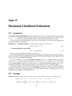
4 Theresult (1) impliesPr n(bp p0)qp0(1 p0) = ,which, after some straightforward calculations, can be shown to be equivalenttoPrhpn p0 pni= +( )2/2 (1 bp)+( )2/4n+( )2pn= +( )2/2+ (1 bp)+( )2/4n+( )24 The intervalhpn,pniis now the 95% confidence interval An application election pollsConsider a presidential election with two candidates, candidateAand can-didateB,and letp0be the fraction of likely voters who favor candidateA,just before the election is held. To predict the outcome of the election, apolling agency draws a random sample of sizen= 3000,for example, fromthe population of likely that1800of the respondents ex-press a preference for candidateA. Thus, the fraction of respondents favoringcandidateAisbp= 3000andbp= the formulasforpnandpnyieldspn= ,pn= , the 95% confidence interval of100 p0is[58,62].The polling resultsare therefore stated as: 60% of the likely voters will vote for candidateA,with a margin of error of Motivation for maximum likelihood esti-mationA more formal motivation for ML estimation is based on the fact that for0<x<1andx>1,ln(x)<x is illustrated in the following picture:1 How to draw such a sample is beyond the scope of this lecture (x) x inequalityln(x)<x 1is strict forx6=1,andln(1) = , takingx=f(Yj|p)/f(Yj|p0),we have the inequalityln f(Yj|p)f(Yj|p0)!

5 F(Yj|p)f(Yj|p0) expectations, it follows thatE"ln f(Yj|p)f(Yj|p0)!# E"f(Yj|p)f(Yj|p0)# 1=f(1|p)f(1|p0)Pr[Yj=1]+f(0|p)f(0|p0)Pr[ Yj=0] 1=pp0p0+1 p1 p0(1 p0) 1=p+1 p 1=0,(2)henceE[ln (f(Yj|p))] E[ln (f(Yj|p0))] =E"ln f(Yj|p)f(Yj|p0)!# 0,and therefore,E[ln (Ln(p))] E[ln (Ln(p0))].(3)Thus,E[ln (Ln(p))]is maximal forp=p0,anditcanbeshownthatthismaximum is maximum likelihood estimation of the The Logit model with one explanatory variableNext, let(Y1,X1), ..,(Yn,Xn)be a random sample from the conditional Logitdistribution:Pr[Yj=1|Xj]=11+exp( 0 0Xj),(4)Pr[Yj=0|Xj]=1 Pr[Yj=1|Xj]=exp ( 0 0Xj)1+exp( 0 0Xj)where theXj s are the explanatory variables and 0and 0are unknownparameters to be estimated. This model is called a Logit model , becausePr[Yj=1|Xj]=F( 0+ 0Xj)(5)whereF(x)=11+exp( x)(6)is the distribution function of the logistic ( Logit ) conditional probability function involved isf(y|Xj, 0, 0)=Pr[Yj=y|Xj]=F( 0+ 0Xj)y(1 F( 0+ 0Xj))1 y=(F( 0+ 0Xj)ify=1,1 F( 0+ 0Xj)ify= the conditional log- likelihood function isln (Ln( , )) =nXj=1ln (f(Yj|Xj, , ))=nXj=1 Yjln (F( + Xj)) +nXj=1(1 Yj)ln(1 F( + Xj))= nXj=1(1 Yj)( + Xj) nXj=1ln (1 + exp ( Xj)).)

6 (7)7 Similar to (3) we haveE[ln(Ln( , ))|X1, .., Xn] E[ln(Ln( 0, 0))|X1, .., Xn].Again, this result motivates to estimate 0and 0by maximizingln (Ln( , ))to and :ln Ln(b ,b ) =max , ln (Ln( , )).However, there is no longer an explicit solution forb andb .These MLestimators have to be solved numerically. Your econometrics software will dothat for Pseudo t-valuesIt can be shown that if the sample sizenis large then n(b 0) N(0, 2 ), n b 0 N(0, 2 ).Given consistent estimatorsb 2 andb 2 of the unknown variances 2 and 2 ,respectively (which are computed by your econometrics software), we thenhave n(b 0)b N(0,1), n b 0 b N(0,1).These results can be used to test whether the coefficients 0and 0are zeroor not. In particular the null hypothesis 0=0is of interest, because thishypothesis implies that the conditional probabilityPr[Yj=1|Xj]does notdepend the null hypothesis 0=0we havebt = nb b N(0,1).Recall that the 5% critical value of the two-sided standard normal test Thus, for example, the null hypothesis 0=0is rejected at the 5%significance level in favor of the alternative hypothesis 06=0if bt > ,andacceptedif bt statisticbt is called thepseudot-value ofb because it is used in thesame way as the t-value in linear regression, andb is called the standarderror ofb.

7 Your econometric software will report the ML estimators togetherwith their corresponding pseudo t-values and/or standard The general Logit modelThe general Logit model takes the formPr[Yj=1|X1j,..Xk,j]=11+exp( 01X1j .. 0kXkj)(8)=11+exp Pki=1 0iXij ,where one of theXijequals 1 for the constant term, for example, letXkj=1,and the 0i s are the true parameter values. This model can be estimated byML in the same way as before. Thus, the log- likelihood function isln (Ln( 1, .., k)) = nXj=1(1 Yj)kXi=1 iXij nXj=1ln 1+exp kXi=1 iXij!!,(9)and the ML estimatorsb 1, ..,b kare obtained by maximizingln (Ln( 1, .., k)):ln Ln(b 1,..,b k) =max 1,.., kln (Ln( 1, .., k)).Again, it can be shown that ifnis large then fori=1, .., k, n b i 0i N[0, 2i].Given consistent estimatorsb 2iof the variances 2i,it follows then that n b i 0i b i N[0,1]fori=1, .., econometrics software will report the ML estimatorsb itogether with their corresponding pseudo t-valuesbti= nb i/b iand/orstandard errorsb Testing joint significanceNow suppose you want to test the joint null hypothesisH0: 01=0, 02=0.

8 , 0m=0,(10)9wherem< are two ways to do that. One way is akin to the F test in linearregression: Re-estimate the Logit model under the null hypothesis:ln Ln(0,..,0,e m+1, ..,e k) =max m+1,.., kln (Ln(0, ..,0, m+1, .., k)).and compare the log-likelihoods2. Itcanbeshownthatunderthenullhy-pothesis (10) and for large samples,LRm= 2ln Ln(0, ..,0,e m+1, ..,e k)Ln(b 1, ..,b k)! 2m,where the degrees of freedommcorresponds to the number of restrictionsimposed under the null hypothesis. This is the so-called likelihood ratio test,which is conducted right-sided. For example, choose the 5% significancelevel, look up in the table of the 2distribution the critical valuecsuchthat for a 2mdistributed random variableZm,Pr[Zm>c]= thenull hypothesis (10) is rejected at the 5% significance level ifLRm>candaccepted ifLRm alternative test of the null hypothesis (10) is the Wald test, which isconducted in the same way as for linear regression the nullhypothesis (10) the Wald test statistic has also a Interpretation of the coefficients of the Marginal effectsConsider the Logit model (5).

9 If 0>0thenPr[Yj=1|Xj]=F( 0+ 0Xj)is an increasing function ofXj:dP[Yj=1|Xj]dXj= ( 0+ 0Xj),whereF0is the derivative of (6):2 Your econometric software will report the log- likelihood function Internationalthe Wald test can be conducted simply by (x)=exp( x)(1 + exp( x))2=1+exp( x)(1 + exp( x))2 1(1 + exp( x))2=11+exp( x) 1(1 + exp( x))2=F(x) F(x)2=F(x)(1 F(x)).Therefore, the marginal effect ofXjonPr[Yj=1|Xj]depends onXj:dP[Yj=1|Xj]dXj= ( 0+ 0Xj)(1 F( 0+ 0Xj)),which renders the Interpretation of , the coefficient 0can be interpreted in terms of relative changesin Odds and odds ratiosThe odds is the ratio of the probability that something is true divided by theprobability that it is not true. Thus, in the Logit case (4),Odds(X)=Pr[Yj=1|Xj]Pr[Yj=0|Xj]=F( 0+ 0Xj)1 F( 0+ 0Xj)=exp( 0+ 0Xj).(11)The odds ratio is the ratio of two odds for different values ofXj,sayXj=xandXj=x+ x:Odds(x+ x)Odds(x)=exp( + x+ x)exp( + x)=exp( x),where xis a small change x 01 x Odds(x+ x) Odds(x)Odds(x)!

10 = lim x 0exp( 0 x) 1 x= 0lim 0 x 0exp( 0 x) 1 0 x= 0 dexp(u)du u=0= 0exp(0) = , 0may be interpreted as therelativechange in the odds due to a smallchange xinXj:Odds(x+ x) Odds(x)Odds(x)=Odds(x+ x)Odds(x) 1 0 x(12)11 IfXjis a binary variable itself,Xj=0orXj=1, then the only reasonablechoices forx+ xandxare 1 and 0, respectively, so that thenOdds(1)Odds(0) 1=Odds(1) Odds(0)Odds(0)=exp( 0) if 0is small we may then use the approximationexp( 0) 1 , one has to interpret 0in terms of the log of the odds ratio involved:ln Odds(1)Odds(0)!= Interpretation of the coefficients 0i,i=1, .., k 1in the generalLogit model (8) is similar as in the case (12):Odds(X1j, .., Xi 1,j,Xi,j+ Xi,j,Xi+1,j, .., Xk,j)Odds(X1j, .., Xi 1,j,Xi,j,Xi+1,j, .., Xk,j) 1 0i Xi,jif Xi,jis small. For example, 0imay be interpreted as the percentagechange in Odds(X1j, .., Xk,j)due to a small percentage change100 Xi,j=1inXi.