Transcription of Lab 9: FTT and power spectra - Claremont Colleges
1 lab 9 : ftt and power spectra The Fast Fourier Transform (FFT) is a fast and efficient numerical algorithm that computes the Fourier transform. The power spectrum is a plot of the power , or variance, of a time series as a function of the frequency1 . If G(f ) is the Fourier transform, then the power spectrum, W (f ), can be computed as W (f ) = |G(f )| = G(f )G (f ). where G (f ) is the complex conjugate of G(f ). We refer to the power spectrum calculated in this way as the periodogram. Currently, many investigators prefer to estimate the power spectral density us- ing (). This method is based on Welch's averaged periodogram method. Welch's method reduces noise in the estimated spectrum at the expense of reducing the frequency resolution (see below). For many of the ex- perimental uses of power spectra , the advantages of reducing the effects of noise out-weigh the dis-advantages of reduced frequency resolution. As we showed in lecture there is little practiacl difference between determining the periodogram versus the power spectral density.
2 However, the flexibility of () pro- vides esufficient motivation to learn how to use this package. Often overlooked is that the fact that W (f ) is the power spectrum obtained for an infinitely long time series measured with infinitely fine precision. In con- trast, in the laboratory we work with time series of finite length that are subjected to uncorrelated, random inputs (noise) and effects introduced by the process of measuring the signal. The purpose of this laboratory is to illustrate the use of () and explore a number of applications of the FFT and power spectra . 1. For simplicity we have assumed that the independent variable is time; however, it could also be a spatial dimension. We use the term power spectra as a collective term to include both the periodogram and the power spectral density. 1. Browser: Essentially everything that you would ever want to know about the uses of the FFT can be located on the Internet by asking the right questions.
3 In Python, the functions necessary to calculate the FFT are located in the numpy library called fft. If we want to use the function fft(), we must add the following command to the top matter of our program: import as fft Thus, the command for determining the FFT of a signal x(t) becomes (x). Of course, you could import the fft-package from numpy under a different name; however, this might make the program less readable by others. Other functions related to the use of the FFT are located in scipy such as the library signal, import as signal The description of each command and how to use it can easily be obtained by us- ing your web browser and typing the name of the library together with the function that you want to know about. House keeping: Today we will illustrate the applications of the FFT and the power spectra by working with real data. The deliverables take the form of fig- ures prepared using Matplotlib. We suggest that you create a directory for each figure which contains both the data and the program(s) used to generate the required figure.
4 This is actually a good habit to acquire. One advantage is that you don't need to worry about specifying the required paths since, by default, a Python program looks first in the directory they are running for required input files. A second advantage occurs if, my goodness, you actually need to modify your figure at a later date following comments made by a grader or a reviewer of your article (senior thesis, publications, book). 1 Background We illustrate the difference between W (f ) and w(f ) by calculating the power spectrum of x(t) = sin(2 f0 t), where f0 is a particular frequency. By definition, the Fourier transform of sin(2 f t) is Z . G(sin 2 f0 t)(f ) = e 2 jf t sin 2 f0 tdt (1).. 2. where we have distinguished a particular value of the frequency, f , as f0 . Using Euler's relation, we can write e2 jf0 t e 2 jf0 t sin 2 f0 t =. 2j Substituting into (1), we obtain . e2 jf0 t e 2 jf0 t Z . 2 jf t G(sin 2 f0 t)(f ) = e dt 2j 1 2 j(f f0 )t Z.
5 E 2 j(f +f0 )t dt . = e 2j . 1. = [ (f f0 ) (f + f0 )]. 2j j = [ (f + f0 ) (f f0 )]. 2. Here we see that both the Fourier transform and the power spectrum, W (f ), of sin(2 f t) are predicted to be composed of two delta-functions, one centered at +f0 and the other at f0 . Figure 1: Computer screen shot obtained after typing python at the Command prompt. The three >>> means that we are operating in script mode. Now let's use Python to compute the FFT and the power spectrum, w(f ). Python can be run directly from the command line, namely in an interactive mode2. (a much more powerful and popular version of interactive Python programming 2. Up to now we have run Python in its script mode, namely, we write computer program, and then run the program by typing python (Did you remember to add the & ?). There are two advantages: 1) we can use the same program over and over again, and 2). the program gives us a permanent record of what we did. However, the interactive mode is useful when the goal is simply to explore data.
6 3. Figure 2: Obtaining the fft of a 1s 4Hz sine wave by running Python in script mode. Note that most of the numbers for the fft are very small: there are two exceptions. See text for discussion. is iPython). To enable the interactive mode type python in your command window (Figure 1). Type the lines of Python code shown in Figure 2 to obtain the FFT of a 1 Hz sine wave. What does the output on the screen mean? First we note that there are 8. numbers (the sin(2 f0 t) was digitized to give 8 data points per second), all of the numbers are written in the form of a complex number, and Python uses the convention that j = 1. By convention the FFT is outputted using reverse- wrap-around ordering. For this example, the ordering of the frequencies is [0, 1, 2, 3, 4, 3, 2, 1]. Note that the 8 discrete data points yield 8 Fourier coefficients and that the highest frequency that will be resolved is the Nyquist frequency, N/2. The first half of the list of numbers corresponds to the positive frequencies and the second half to the negative frequencies.
7 We suspect that most of you expected to see on the computer screen 4. + However, notice that many of the numbers are very, very small, for example of the order 10 17 . These numbers simply represent numerical noise in the computer. If we set mentally all numbers < 10 3 equal to 0, then we obtain the expected result. It should be noted that recent releases of include the commands rfft() and irfft(). The advantage of using rfft() over fft() becomes of practical importance when we consider a problem that can arise when we com- pute the inverse FFT using ifft(). Since we typically have a real signal, we expect that the inverse should also be real. However, it can happen, due to round- ing errors, that ifft() contains complex numbers. The use of rfft() avoids this problem. Thanks to the development of computer software packages, such as MATLAB, Mathematica, Octave and Python, this task has become much easier. A particu- larly useful function is Python's () developed by the late John D.
8 Hunter3. (x, NFFT, Fs, detrend, window, noverlap=0, pad_to, sides=, scale_by_freq). It is important to keep in mind that psd() does not calculate the periodogram, but calculates the power spectral density using a mathematical method known as Welch's method. The advantages of using () are that it is very versatile and for everyday use we can accept the default choices for most of the options. 2 Exercise 1: Computing the power spectral density using (). power Spectral Density Recipe In the not too distant past, obtaining proper power spectra was a task that was beyond the capacity of most biologists4 . However, thanks to the development 3. We strongly recommend that readers do not use pylab's version of psd(). The mat- () produces the same power spectrum as obtained using the corresponding pro- grams in MATLAB. 4. For convenience we reproduce Section here. 5. Figure 3: a) One-sided periodogram computed for 1s of a 4Hz sine wave using (1). b) One-sided power spectral density computed using () for the same signal used in a).
9 Of computer software packages such as MATLAB, Mathematica, Octave, and Python, this task has become much easier. Although it is relatively easy to write a computer program that computes the periodogram, it is not so easy to write the program in a manner that is convenient for many of the scenarios encountered by an experimentalist. For this reason we strongly recommend the use of Python's (), developed by the late John D. Hunter using the method described by Bendat and Piersol [1].5 This function has the form power , freqs = (x, NFFT, Fs, detrend, window, noverlap=0, pad_to, sides=, scale_by_freq). 5. Do not use PyLab's version of psd(). The function () produces the same power spectrum as that obtained using the corresponding programs in MATLAB. 6. The output is two one-dimensional arrays, one of which gives the values of the power in db Hz 1 , the other the corresponding values of the frequency. The advantage of () is its versatility. Assuming that an investigator has available a properly low-pass-filtered time signal, the steps for obtaining the power density density are as follows: 1.
10 Enter the filtered and discretely sampled time signal x(t). 2. The number of points per data block is NFFT. NFFT must be an even num- ber. The computation is most efficient if NFFT = 2n , where n a positive integer; however, with modern laptops, the calculations when NFFT 6= 2n are performed quickly. 3. Enter Fs. This parameter scales the frequency axis on the interval [0, F s/2], where F s/2 is the Nyquist frequency. 4. Enter the detrend option. Recall that it this a standard procedure to remove the mean from the time series before computing the power spectrum. 5. Enter the windowing option. Keep in mind that using a windowing function is better than not using one, and from a practical point of view, there is little difference among the various windowing functions. The default is the Hanning windowing function. 6. Typically accept the overlap default choice of 0 (see below for more details). 7. Choose pad to (see below). The default is 0.