Transcription of Excel 2016 Intermediate Quick Reference - CustomGuide
1 2021 CustomGuide , Inc. Click the topic links for free lessons! Contact Us: Chart Elements Microsoft Excel 2016 Intermediate Quick Reference GuideCharts Create a Chart: Select the cell range that contains the data you want to chart. Click the Insert tab on the ribbon. Click a chart type button in the Charts group and select the chart you want to insert. Move or Resize a Chart: Select the chart. Place the cursor over the chart s border and, with the 4-headed arrow showing, click and drag to move it. Or, click and drag a sizing handle to resize it. Change the Chart Type: Select the chart and click the Design tab. Click the Change Chart Type button and select a different chart.
2 Filter a Chart: With the chart you want to filter selected, click the Filter button next to it. Deselect the items you want to hide from the chart view and click the Apply button. Position a Chart s Legend: Select the chart, click the Chart Elements button, click the Legend button, and select a position for the legend. Show or Hide Chart Elements: Select the chart and click the Chart Elements button. Then, use the check boxes to show or hide each element. Insert a Trendline: Select the chart where you want to add a trendline. Click the Design tab on the ribbon and click the Add Chart Element button. Select Trendline from the menu. Charts Insert a Sparkline: Select the cells you want to summarize.
3 Click the Insert tab and select the sparkline you want to insert. In the Location Range field, enter the cell or cell range to place the sparkline and click OK. Create a Dual Axis Chart: Select the cell range you want to chart, click the Insert tab, click the Combo button, and select a combo chart type. Print and Distribute Set the Page Size: Click the Page Layout tab. Click the Size button and select a page size. Set the Print Area: Select the cell range you want to print. Click the Page Layout tab, click the Print Area button, and select Set Print Area. Print Titles, Gridlines, and Headings: Click the Page Layout tab. Click the Print Titles button and set which items you wish to print.
4 Add a Header or Footer: Click the Insert tab and click the Header & Footer button. Complete the header and footer fields. Adjust Margins and Orientation: Click the Page Layout tab. Click the Margins button to select from a list of common page margins. Click the Orientation button to choose Portrait or Landscape orientation. Column: Used to compare different values vertically side-by-side. Each value is represented in the chart by a vertical bar. Line: Used to illustrate trends over time (days, months, years). Each value is plotted as a point on the chart and values are connected by a line. Pie: Useful for showing values as a percentage of a whole when all the values add up to 100%.
5 The values for each item are represented by different colors. Bar: Similar to column charts, except they display information in horizontal bars rather than in vertical columns. Area: Similar to line charts, except the areas beneath the lines are filled with color. XY (Scatter): Used to plot clusters of values using single points. Multiple items can be plotted by using different colored points or different point symbols. Stock: Effective for reporting the fluctuation of stock prices, such as the high, low, and closing points for a certain day. Surface: Useful for finding optimum combinations between two sets of data. Colors and patterns indicate values that are in the same range.
6 Chart Options Chart Types Additional Chart Elements Data Labels: Display values from the cells of the worksheet on the plot area of the chart. Data Table: A table added next to the chart that shows the worksheet data the chart is illustrating. Error Bars: Help you quickly identify standard deviations and error margins. Trendline: Identifies the trend of the current data, not actual values. Can also identify forecasts for future data. Chart Title Data Bar Chart Area Axis Titles Legend Chart Elements Chart Styles Chart Filters Gridline Free Cheat SheetsVisit 2021 CustomGuide , Inc. Click the topic links for free lessons! Contact Us: Intermediate Formulas Absolute References: Absolute references always refer to the same cell, even if the formula is moved.
7 In the formula bar, add dollar signs ($) to the Reference you want to remain absolute (for example, $A$1 makes the column and row remain constant). Name a Cell or Range: Select the cell(s), click the Name box in the Formula bar, type a name for the cell or range, and press Enter. Names can be used in formulas instead of cell addresses, for example: =B4*Rate. Reference Other Worksheets: To Reference another worksheet in a formula, add an exclamation point ! after the sheet name in the formula, for example: =FebruarySales!B4. Reference Other Workbooks: To Reference another workbook in a formula, add brackets [ ] around the file name in the formula, for example: =[ ]Sheet1!$B$4.
8 Order of Operations: When calculating a formula, Excel performs operations in the following order: Parentheses, Exponents, Multiplication and Division, and finally Addition and Subtraction (as they appear left to right). Use this mnemonic device to remember them: Please Parentheses Excuse Exponents My Multiplication Dear Division Aunt Addition Sally Subtraction Concatenate Text: Use the CONCAT function =CONCAT(text1,text2,..) to join the text from multiple cells into a single cell. Use the arguments within the function to define the text you want to combine as well as any spaces or punctuation. Payment Function: Use the PMT function =PMT(rate,nper,pv,..) to calculate a loan amount.
9 Use the arguments within the function to define the loan rate, number of periods, and present value and Excel calculates the payment amount. Date Functions: Date functions are used to add a specific date to a cell. Some common date functions in Excel include: Date =DATE(year,month,day) Today =TODAY() Now =NOW() Display Worksheet Formulas: Click the Formulas tab on the ribbon and then click the Show Formulas button. Click the Show Formulas button again to turn off the formula view. Manage Data Export Data: Click the File tab. At the left, select Export and click Change File Type. Select the file type you want to export the data to and click Save As. Import Data: Click the Data tab on the ribbon and click the Get Data button.
10 Select the category and data type, and then the file you want to import. Click Import, verify the preview, and then click the Load button. Use the Quick Analysis Tools: Select the cell range you want to summarize. Click the Quick Analysis button that appears. Select the analysis tool you want to use. Choose from formatting, charts, totals, tables, or sparklines. Outline and Subtotal: Click the Data tab on the ribbon and click the Subtotal button. Use the dialog box to define which column you want to subtotal and the calculation you want to use. Click OK. Use Flash Fill: Click in the cell to the right of the cell(s) where you want to extract or combine data. Start typing the data in the column.