Transcription of Lumped and Consistent Mass Matrices - Quickfem
1 31 LumpedandConsistentMassMatrices31 1 chapter 31: Lumped AND Consistent MASS MATRICES31 2 TABLE OF CONTENTSPage 3 Matrix Construction31 3 Direct Mass 3 Variational Mass 4 Template Mass 4 Mass Matrix 5 Ran kand Numerical 6 6 Matrix Examples: Bars and Beams31 8 The 3-Node 8 The Bernoulli-Euler Plane 8 The Plane 10 *The Timoshenko Plane 11 Spar and Shaft 12 Matrix Examples: Plane Stress31 12 The Plane Stress Linear 12 Four-Node Bilinear 14 Diagonalization Methods31 15 HRZ 15 Lobatto 15 and 16 18 1931 231 3 MASS MATRIX CONSTRUCTION IntroductionTo do dynamic and vibration finite element analysis, you need at least a mass matrix to pair withthe stiffness matrix. This chapter provides a quic kintroduction to standard methods for computingthis a general rule, the construction of the master mass matrixMlargely parallels of the masterstiffness matrixK. Mass Matrices for individual elements are formed in local coordinates, trans-formed to global, and merged into the master mass matrix following exactly the same techniquesused forK.
2 In practical terms, the assemblers forKandMcan be made identical. This proceduraluniformity is one of the great assets of the Direct Stiffness notable difference with the stiffness matrix is the possibility of using adiagonalmass matrixbased on direct lumping. A master diagonal mass matrix can be stored simply as a vector. If allentries are nonnegative, it is easily inverted, since the inverse of a diagonal matrix is also a Lumped mass matrix entails significant computational advantages for calculations thatinvolveM 1. This is balanced by some negative aspects that are examined in some detail later. Mass Matrix ConstructionThe master mass matrix is built up from element contributions, and we start at that level. Theconstruction of the mass matrix of individual elements can be carried out through several can be categorized into three groups: direct mass lumping, variational mass lumping, andtemplate mass lumping. The last group is more general in that includes all others.
3 Variants ofthe first two techniques are by now standard in the FEM literature, and implemented in all generalpurpose codes. Consequently this chapter covers the most widely used methods, focusing ontechniques that produce diagonally Lumped and Consistent mass Matrices . The next chapter coversthe template approach to produce customized mass Matrices . Direct Mass LumpingThe total mass of elementeis directly apportioned to nodal freedoms, ignoring any cross goal is to build adiagonally Lumped mass matrixor DLMM, denoted here the simplest example, consider a 2-node prismatic barelement with length , cross section areaA, and mass density , which can only move in the axial directionx, as depictedin Figure The total mass of the element isMe= A .This is divided into two equal parts and assigned to each endnode to produceMeL=12 A 1001 =12 A I2,( )massless connectorTotal mass A A A Direct mass lumping for2-node prismatic bar whichI2denotes the 2 2 identity matrix. As shown in the figure, we have replaced the barwith a dumbbell.
4 This process conserves the translational kinetic energy or, equivalently, the linear momentum. Toshow this for the bar example, take the constantx-velocity vector ue=v[11]T. The kinetic31 3 chapter 31: Lumped AND Consistent MASS MATRICES31 4energy of the element isTe=12( ue)TMeL ue=12 A v2=12 Mev2. Thus the linear momentumpe= Te/ v=Mevis preserved. When applied to simple elements that can rotate, however, thedirect lumping process may not necessarily key motivation for direct lumping is that, as noted in , a diagonal mass matrix may offercomputational and storage advantages in certain simulations, notably explicit time , direct lumping covers naturally the case where concentrated (point) masses are naturalpart of model building. For example, in aircraft engineering it is common to idealize nonstructuralmasses (fuel, cargo, engines, etc.) as concentrated at given Variational Mass LumpingA second class of mass matrix construction methods are based on a variational formulation.
5 Thisis done by taking thekinetic energyas part of the governing functional. The kinetic energy of anelement of mass density that occupies the domain eand moves with velocity field veisTe=12 e ( ve)T ved e.( )Following the FEM philosophy, the element velocity field is interpolated by shape functions: ve=Nev ue, where ueare node DOF velocities andNeva shape function matrix. Inserting into ( ) andmoving the node velocities out of the integral givesTe=12( ue)T e (Nev)TNevd uedef=12( ue)TMe ue,( )whence the element mass matrix follows as the Hessian ofTe:Me= 2Te ue ue= e (Nev)TNevd .( )If the same shape functions used in the derivation of the stiffness matrix are chosen, that is,Nev=Ne,( ) is called theconsistent mass matrix2or CMM. It is denoted here the 2-node prismatic bar element moving alongx, the stiffness shape functions of chapter 12areNi=1 (x xi)/ =1 andNj=(x xi)/ = . Withdx= d , the Consistent mass iseasily obtained asMeC= 0 A(Ne)TNedx= A 10 1 [1 ] d =16 A 2112.
6 ( )It can be verified that this mass matrix preserves linear momentum concentrated masses in general have rotational freedoms. Rotational inertia lumping is then part of the better name would be stiffness- Consistent . The shorter sobricket has the unfortunately implication that other choices are inconsistent, which is far from the truth. In fact, the Consistent mass is not necessarily the best one, a topic elaboratedin the next chapter . However the name is by now ingrained in the FEM 431 5 MASS MATRIX CONSTRUCTION Template Mass LumpingA generalization of the two foregoing methods consists of expressing the mass as a linear combi-nation ofkcomponent mass Matrices :Me= ki=1 iMei.( )Appropriate constraints on the free parameters iare placed to enforce matrix properties discussedin Variants result according to how the component matricesMiare chosen, and how theparameters iare determined. The best known scheme of this nature results on taking a weightedaverage of the Consistent and diagonally- Lumped mass Matrices :MeLCdef=(1 )MeC+ MeL,( )in which is a free scalar parameter.
7 This is called the LC ( Lumped - Consistent ) weighted massmatrix. If =0 and =1 this combination reduces to the Consistent and Lumped mass matrix,respectively. For the 2-node prismatic bar we getMeLC=(1 )16 A 2112 + 12 A 1001 =16 A 2+ 1 1 2+ .( )It is known (since the early 1970s) that the best choice with respect to minimizing low frequencydispersion is = / . This is proven in the next most general method of this class usesfinite element templatesto fully parametrize the elementmass matrix. For the prismatic 2-node bar element one would start with the 3-parameter templateMe= A 11 12 12 22 ,( )which includes the symmetry constraint from the start. Invariance requires 22= 11, which cutsthe free parameters to two. Conservation of linear momentum requires 11+ 12+ 12+ 22=2 11+2 12=1, or 12= / 11. Taking =6 11 2 reduces ( ) to ( ). Consequentlyfor the 2-node bar LC-weighting and templates are the same thing, because only one free parameteris left upon imposing essential constraints.
8 This is not the case for more complicated elements. Mass Matrix PropertiesMass Matrices must satisfy certain conditions that can be used for verification and debugging. Theyare: (1) matrix symmetry, (2) physical symmetries, (3) conservation and (4) Symmetry. This means(Me)T=Me, which is easy to check. For a variationally derivedmass matrix this follows directly from the definition ( ), while for a DLMM is Symmetries. Element symmetries must be reflected in the mass matrix. For example, theCMM or DLMM of a prismatic bar element must be symmetric about the antidiagonal:M11= see this, flip the end nodes: the element remains the same and so does the mass 5 chapter 31: Lumped AND Consistent MASS MATRICES31 6 Conservation. At a minimum, total element mass must be is easily verified byapplying a uniform translational velocity and checking that linear momentum is conserved. Higherorder conditions, such as conservation of angular momentu, are optional and not always For any nonzero velocity field defined by the node values ue =0,( ue)TMe ue 0.
9 Thatis,Memust be nonnegative. Unlike the previous three conditions, this constraint is nonlinear in themass matrix entries. It can be checked in two ways: through the eigenvalues ofMe, or the sequenceof principal minors. The second technique is more practical if the entries ofMeare A more demanding form of the positivity constraint is to require thatMebepositive definite:( ue)TMe ue>0 for any ue =0. This is more physically reassuring because one half of that quadratic formis the kinetic energy associated with the velocity field defined by ue. In a continuumTcan vanish only forzero velocities. But allowingTe=0 for some nonzero uemakes life easier in some situations, particularlyfor elements with rotational or Lagrange multiplier uefor whichTe=0 form thenull spaceofMe. Because of the conservation requirement, a rigid velocityfield (the time derivative ueRof a rigid body modeueR) cannot be in the mass matrix null space, since it wouldimply zero mass. This scenario is dual to that of the element stiffness matrix.
10 For the latter,KeueR=0, sincea rigid body motion produces no strain energy. ThusueRmust be in the null space of the stiffness matrix. Rank and Numerical IntegrationSuppose the element has a total ofneFfreedoms. A mass matrixMeis calledrank sufficientor offull rankif its ran kisreM=neF. Because of the positivity requirement, a rank-sufficient mass matrixmust be positive definite. Such Matrices are preferred from a numerical stability rankreM<neFthe mass is called ran kdeficient bydeM=neF reM. EquivalentlyMeisdeMtimes singular. For a numerical matrix the ran kis easily computed by ta king its eigenvaluesand looking at how many of them are zero. The null space can be extracted by functions such asNullSpaceinMathematicawithout the need of computing computation ofMeby the variational formulation ( ) is often done using Gauss numericalquadrature. Each Gauss points addsnDto the rank, wherenDis the row dimension of the shapefunction matrixNe, up to a maximum ofneF. For most elementsnDis the same as element spatialdimensionality; that is,nD=1, 2 and 3 for 1, 2 and 3 dimensions, respectively.