Transcription of CHAPTER 6 INTRODUCTION TO SYSTEM …
1 CHAPTER 6 introduction to system identification Broadly speaking, SYSTEM identification is the art and science of using measurements obtained from a SYSTEM to characterize the SYSTEM . The characterization of the SYSTEM is usually in some mathematical form. The limited cases considered here will use differential equations, in particular, first and second order differential equations. When the form of the differential equation is known the SYSTEM identification problem is reduced to that of parameter identification .
2 Present industrial practice presents several situations where SYSTEM identification is used. An important application is in industrial controls. Before a controller can be designed some things must be known about the SYSTEM which is to be controlled. Many systems do not lend themselves to modeling and the most effective way to find out about the SYSTEM is to make measurements and apply the methods of SYSTEM identification . The use of the methods covered in this course and even more sophisticated methods such as finite element methods for modeling real engineering systems, even simple ones, yield only approximate results and the models must be adjusted using data obtained from the SYSTEM .
3 For most mechanical systems there are no analytical methods for predicting SYSTEM damping so that engineering judgment or SYSTEM identification methods must be used. The measurements which are used for SYSTEM identification can arise in one of several ways. For large systems such as a building, ambient data is used. That is, natural excitations such as wind, are used to excite the SYSTEM . Even for uncontrolled random excitations such as this, spectra that show the average distribution of response signal power as a function of frequency can be used to identify SYSTEM characteristics.
4 These methods will not be discussed further here. We will use several controlled inputs to give SYSTEM responses which are easier to analyze. These would include a step input (such as a sudden change in temperature of a thermo SYSTEM ), a snap back (such as deflecting a spring-mass SYSTEM and then suddenly releasing it), an impulse (such as striking a spring-mass SYSTEM with a sharp blow), or sinusoidal input. The selection of which input to use is a function of your ability to generate the input and record and analyze the response.
5 These notes will only cover 1st and 2nd order systems. Real engineering systems are rarely 1st or 2nd order systems so the practical utility of these simple systems is questionable. Fortunately, from an analysis point of view, even complex mechanical systems can be represented by several connected first and second order systems. Consider as an example the measurement SYSTEM shown in Figure 1. The first component is an accelerometer which is a second order SYSTEM , it is connected to an amplifier which is a first order SYSTEM , and a recording device which can be 6-2 modeled as a second order SYSTEM .
6 The total measurement SYSTEM is thus fifth order but can be modeled as three simpler systems connected in series. acceleration deflection Figure 1: A simple SYSTEM for measuring acceleration. Having identified models of the SYSTEM sub-components, they can be combined to form a model of the entire SYSTEM . This is not always straightforward because systems interact when they are connected.
7 Interaction between sub-components is discussed in the next CHAPTER . At the end of the last CHAPTER we showed how to combine descriptions of sub- SYSTEM behavior to form a description of the total SYSTEM behavior, for the case when the interaction effects can be ignored. In this case, often encountered in practice because measurement SYSTEM sub-components are usually designed to virtually eliminate these interaction effects, the derivation of the total SYSTEM model from the sub-component models is very straightforward.
8 So while the systems and methods that we look at in detail in this CHAPTER are fairly simple, by breaking down a complicated SYSTEM into simpler sub-components, we can use these SYSTEM identification methods to identify characteristics of more complicated systems. Thus, these simple methods are also often used by industry. accelerometer 2nd Order amplifier 1st Order recorder 2nd Order 6-3 First Order Systems: The differential equation is given by y(t) y(t)K x(t) (1) where y(t) is the SYSTEM response x(t) is the excitation is the time constant, an indication of how fast the SYSTEM responds K is the static sensitivity.
9 Thermocouples, amplifiers, resistance temperature devices and RC circuits are examples of systems whose behavior can be modeled with a first order differential equation such as equation (1 ). Step Response of a First Order SYSTEM Consider first the step response, that is, the response of the SYSTEM subjected to a sudden change in the input which is then held constant. sx(t) Cu (t) where C is the magnitude of the step. su (t) is the unit step function defined below, ssu (t) 0 for t 0, and u (t) 1 for t 0 Assume that the SYSTEM is at rest at time t = 0, , y(0) = 0y.
10 As t gets large, fy(t)y, its final value. By solving the differential equation, the response after the step was input is found to be: ttfoy(t)y 1 ey e (2) This can be written in the form: oftfyyy(t)ye steady state initial condition or response transient response Note that if x(t) = 0 the response is that of a SYSTEM with just the initial condition of oy(0) y.