Chapter 3 Frequency Distributions - psy210.faculty.unlv.edu

1 Frequency Distributions Distributions as Tables Distributions as GraphsHistogram Frequency Polygon Eyeball-estimation The Shape of DistributionsDescribing Distributions The Normal distribution Eyeball-calibration Bar Graphs of Nominal and Ordinal Variables ConnectionsCumulative Review Computers Homework Tips Exercises for Chapter 3 Personal Trainer LECTLET 3A: Frequency Distributions as Tables LECTLET 3B: Frequency Distributions as Graphs LABS: Lab for Chapter 3 REViEwMASTER 3A: RESOuRCE 3A: Stem and Leaf Displays RESOuRCE 3X: Additional 336/7/17 4:03 PM34 Chapter 3 Frequency DistributionsLearning Objectives How is a tabular Frequency distribution constructed?

2 What are class intervals and what role do they play in the development of grouped Frequency Distributions ? What are two graphical methods of representing interval/ratio data from grouped Frequency Distributions ? What steps are involved in eyeball-estimating Frequency Distributions ? How are these terms used to describe the shape of Distributions : unimodal, bimodal, symmetric, positively skewed, negatively skewed, asymptotic, normal? How is a bar graph similar to and different from a histogram? For what kind of data is each used?There are three main concepts in statistics: Frequency Distributions , the distribution of the means, and the test statistic.

3 Here we focus on Frequency Distributions and how they are displayed: in tables (as ungrouped and grouped Frequency Distributions ) and in graphs (as histograms and Frequency poly-gons). You will learn to eyeball-estimate Frequency Distributions and terminology for describing the shapes of Distributions : unimodal, bimodal, sym metric, positively and negatively skewed, asymptotic, and shows the grouped Frequency Distributions and Figure shows the his-tograms for the intellectual growth scores in the Pygmalion study of Chapter 1, where Rosenthal and Jacobson (1968) led teachers to believe that bloomers would show IQ spurts, but that other children would not spurt.

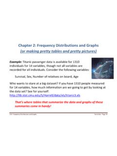
4 Ac tually, the bloomers were a ran-dom sample of students no different, on average, from the other children. The grouped Frequency Distributions (Table ) and histograms (Figure ) show that the most frequently occurring IQ gain among the bloomers was between 11 and 20 IQ points, whereas the most frequently occurring IQ gain among the other children was between 1 and 10 IQ points. It is also easy to see that there is considerable overlap between the bloomer and other children s intellectual GainBloomersOthers 61 70 1 0 51 60 0 0 41 50 0 0 31 40 0 1 21 30 2 2 11 20 614 1 10 118 9 0 2 9 19 10 0 31247*Based on Rosenthal & Jacobson (1968)TaBle Grouped Frequency Distributions of intellectual growth (IQ gain) for Oak School bloomers and other children* Frequency distributionenumeration (ee NEW mer A shun)histogramfrequency polygonunimodal (YOU ni MO dull)

5 Bimodal (BYE MO dull)symmetricskewedasymptotic (ASS sim TOT tic)normalbar 346/7/17 4:03 PM Chapter 3 Frequency Distributions 3520 15 10 5 0 20 - 11 10 - 1 20 - 11 10 - 10-910-1920-29 30-3940-4950-59 60-690-910-1920-29 30-3940-4950-59 60-69 fIQ Gain of Bloomers20 15 10 5 0 fIQ Gain of OthersFIGURe Histograms of intellectual growth (IQ gain) for Oak School bloomers and other children (Based on Rosenthal & Jacobson, 1968)The break in the X-axis shows that the Y-axis does not intersect at X = 0 as is could have made the same observations by inspecting the data in Chapter 1, but the Frequency Distributions described this Chapter make it that in Chapter 1 we pointed out the three major concepts in statistics: (1) what a distribution of a variable is and how to describe it, (2) what a distribution of means is and how it is related to the distribution of a variable, and (3) what a test statistic is and how it is related to the distribution of means.

6 This Chapter (and also Chapters 4 and 5) focuses on (1) the Distributions of variables. Our first task is to convince ourselves that understanding Frequency Distributions will make it simpler for us to think about and communicate about data. Suppose, for example, that we are interested in the weights of male students in our statistics class. There are 25 men in the class, and we measure each man s weight, with the results shown in Figure , where each man is represented by a 356/7/17 4:03 PM36 Chapter 3 Frequency Distributions 135 180 190 137 154 149 164 185 173 163 162 157 161 173 180 179 197 159 182 164 164 144 152 150 163 FIGURe Weights (lb) of male students as they sit in the classroomTaBle Enumeration of male students weights (lb)135180190137154149164185173163162157 161173180179197159182164164144152150163I n an enumerated list, you have to hunt for the largest or smallest suppose our friend Jack asks how heavy the male students in our class are.

7 We could simply list the data: The first student weighs 135 pounds, the next student weighs 180 pounds, the third student weighs .. , and the last student weighs 163 pounds. This kind of listing is called an can be printed, as shown in Table An enumeration is a perfectly accurate answer to Jack s question about student weights, but it is probably an undesir-able answer both because it is too long (we give Jack more information than he wants) and because it does not highlight the important characteristics of the distribution (it does not, for example, make it easy to discover the largest or the smallest weight, or to see which weights occur most frequently).

8 Statisticians make the answers to questions such as Jack s more informative by using Frequency Distributions in the form of tables or Lectlets and then 3A in the Personal Trainer for an audiovisual discussion of Sec tions and Distributions as TablesA tabular Frequency distribution is a table that lists the numerical values of a vari-able in a logical order along with Frequency of each value. A variable, as we saw in Chapter 2, is that characteristic of interest that can take on dif ferent values for each enumeration Listing all points in a data settabular Frequency distribution An ordered listing of all values of a variable and their frequenciesPersonal TrainerLectletsenumeration (ee NEW mer A shun) 366/7/17 4:03 PM Distributions as Tables 37participant, and the Frequency (usually abbreviated f) is the number of times a par-ticular value of the variable occurs.

9 Table shows the tabular Frequency distribu-tion of male students weights. The value 180 occurs twice ( has Frequency 2 ), as do 173 and 163, and the value 164 occurs three times ( has Frequency 3 ). All other frequencies for the weights listed in the table are 1. If a weight does not occur in the data of Table (for example, 181 or 142), then its Frequency is 0, and we omit it entirely in the Table Frequency that the sum of the frequencies (25 in our example) is shown at the bottom of the Frequency column and is always equal to the number of entries in the original data also that the Frequency distribution shows the values of the variable under con sideration (weight) in order; the convention is to put the largest value first.

10 This presentation sim plifies our communication about the data. Now if Jack wants to know how heavy the men in our class are, we can immediately say, The lightest is 135 pounds, the second lightest is 137 pounds, the third lightest is 144 pounds, .. , and the heaviest is 197 pounds. This is still a long and cumbersome answer, but the ordering makes it easier for Jack to gain some appreciation of how the weights stand in relation to each other. However, although this Frequency distribution is more informative than a simple enumeration of the individual weights, it has disadvantages: It still provides a long list of weights and their frequencies, and it is relatively difficult to identify weights with 0 grouped Frequency distribution (also called a Frequency distribution using class intervals ) is more compact and efficient.