Fourier Trans Form
Found 7 free book(s)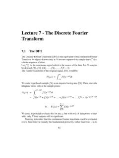
Lecture 7 -The Discrete Fourier Transform
www.robots.ox.ac.ukThe Discrete Fourier Transform (DFT) is the equivalent of the continuous Fourier Transform for signals known only at instants separated by sample times (i.e. a finite sequence of data). Let be the continuous signal which is the source of the data. Let samples be denoted . The Fourier Transform of the original signal,, would be ...
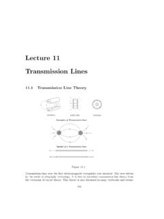
Lecture 11 Transmission Lines - Purdue University
engineering.purdue.edudomain data by performing a Fourier inverse transform. For a time-harmonic signal on a transmission line, one can analyze the problem in the frequency domain using phasor technique. A phasor variable is linearly proportional to a Fourier transform variable. The telegrapher’s equations (11.1.6) and (11.1.7) then become d dz V(z;!) = j!LI(z ...
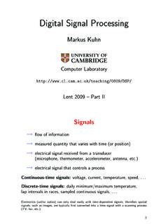
Digital Signal Processing - University of Cambridge
www.cl.cam.ac.ukFourier transform. Harmonic phasors as orthogonal base functions. Forms of the Fourier transform, convolution theorem, Dirac’s delta function, impulse combs in the time and frequency domain. Discrete sequences and spectra. Periodic sampling of continuous signals, pe-riodic signals, aliasing, sampling and reconstruction of low-pass and band-pass
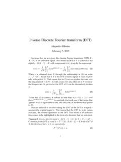
Inverse Discrete Fourier transform (DFT)
www.seas.upenn.edueasier to interpret, say the DFT X, we can compute the respective trans-form and proceed with the analysis. This analysis will neither introduce spurious effect, nor miss important features. Since both representations are equivalent, it is just a matter of which of the representations makes the identification of patterns easier.

Complex Signals - DTU
bme.elektro.dtu.dkwhere x∗(t) is the complex conjugate of x(t), and (↔) denotes a Fourier trans-form pair. Let the complex signal x(t) be expressed in the form: x(t) = x 1(t)+jx 2(t), (2.8) where x 1(t) and x 2(t) are real signals. Let their spectra be X 1(f) and X 2(f), respectively, i.e. x 1(t) ↔ X 1(f) and x 2(t) ↔ X 2(f). The real part of x(t) can be ...
Solutions to Exercises
link.springer.comAn Introduction to Laplace Transforms and Fourier Series 1 1 1 9s 9(s + 3) 3(s + 3)2 ~ -~(3t + 1)e-3t 99· (d) This last part is longer than the others. The partial fraction decom position is best done by computer algebra, although hand computation is possible. The result is 1 1 3 1 2
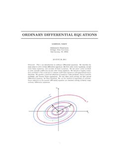
ORDINARY DIFFERENTIAL EQUATIONS
users.math.msu.eduWe introduce Laplace trans-form methods to nd solutions to constant coe cients equations with generalized source functions. We provide a brief introduction to boundary value problems, Sturm-Liouville problems, and Fourier Series expansions. We end these notes solving our rst partial di erential equation, the Heat Equation. We use the method of ...