Search results with tag "Zernike"
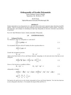
Orthogonality of Zernike Polynomials - Sigmadyne
www.sigmadyne.comThe “Standard Zernike” polynomials as defined above have a value of 1.0 at ρ=1. CodeV uses this normalization. The surface RMS of each CodeV unit Zernike polynomial is:

Optical Design with Zemax for PhD - Basics
www.iap.uni-jena.de4 13.11. Aberrations I representations, spot, Seidel, transverse aberration curves, Zernike wave aberrations 5 20.11. Aberrations II Point spread function and transfer function 6 27.11. Optimization I algorithms, merit function, variables, pick up’s 7 04.12. Optimization II methodology, correction process, special requirements, examples 8 11.12.

Introduction to ISO 10110 - University of Arizona
wp.optics.arizona.edu• One comment on Zernike polynomials – The standard uses the FRINGE monomial p-v ordering – I think this is short sighted – You should use double indices as in – Where I is the power of the radial parameter, and – j is the angular order j α i
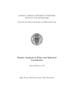
Fourier Analysis in Polar and Spherical Coordinates
lmb.informatik.uni-freiburg.deThe Zernike polynomials are a set of orthogonal polynomials defined on a unit disk, which have the same angular part as (4). The SH transform works on the spherical surface. When it is used for 3D volume data, the SH features (extracted from SH coefficients) can be calculated
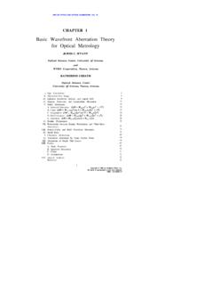
Basic Wavefront Aberration Theory for Optical Metrology
wyant.optics.arizona.eduZernike polynomials have three properties that distinguish them from other sets of orthogonal polynomials. First, they have simple rotational symmetry properties that lead to a polynomial product of the form (49) where G (θ′ ) is a continuous function that …

Spatial & Temporal Coherence - NTUA
users.ntua.grvan Cittert-Zernike Theorem states that the spatial coherence area A c is given by: where d is the diameter of the light source and D is the distance away. Basically, wave -fronts smooth . out as they propagate away ; from the source. Prof. Elias N. Glytsis, School of ECE, NTUA ; 15 .
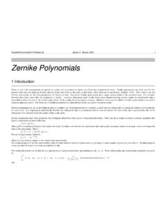
Zernike Polynomials - University of Arizona
wp.optics.arizona.eduZernike Polynomials 1 Introduction Often, to aid in the interpretation of optical test results it is convenient to express wavefront data in polynomial form. Zernike polynomials are often used for this purpose since they are made up of terms that are of the same form as the types of aberrations often observed in optical tests (Zernike, 1934).