Transcription of 1.0 The Admittance Matrix C - Iowa State University
1 The Power Flow equations The Admittance Matrix Current injections at a bus are analogous to power injections. The student may have already been introduced to them in the form of current sources at a node. Current injections may be either positive (into the bus) or negative (out of the bus). Unlike current flowing through a branch (and thus is a branch quantity), a current injection is a nodal quantity. The Admittance Matrix , a fundamental network analysis tool that we shall use heavily, relates current injections at a bus to the bus voltages. Thus, the Admittance Matrix relates nodal quantities. We motivate these ideas by introducing a simple example.
2 We assume that all electrical variables in this document are given in the per-unit system. Fig. 1 shows a network represented in a hybrid fashion using one- line diagram representation for the nodes (buses 1-4) and circuit representation for the branches connecting the nodes and the branches to ground. The branches connecting the nodes represent lines. The branches to ground represent any shunt elements at the buses, including the charging capacitance at either end of the line. All branches are denoted with their Admittance values yij for a branch connecting bus i to bus j and yi for a shunt element at bus i. The current injections at each bus i are denoted by Ii.
3 1 y13 3 4. I1 y34. 2 I4. y12 y23. I2 I3. y1 y4. y2 y3. Fig. 1: Network for Motivating Admittance Matrix 1. Kirchoff's Current Law (KCL) requires that each of the current injections be equal to the sum of the currents flowing out of the bus and into the lines connecting the bus to other buses, or to the ground. Therefore, recalling Ohm's Law, I=V/z=Vy, the current injected into bus 1 may be written as: I1=(V1-V2)y12 + (V1-V3)y13 + V1y1 (1). To be complete, we may also consider that bus 1 is connected to bus 4 through an infinite impedance, which implies that the corresponding Admittance y14 is zero. The advantage to doing this is that it allows us to consider that bus 1 could be connected to any bus in the network.
4 Then, we have: I1=(V1-V2)y12 + (V1-V3)y13 + (V1-V4)y14 + V1y1 (2). Note that the current contribution of the term containing y14 is zero since y14 is zero. Rearranging eq. 2, we have: I1= V1( y1 + y12 + y13 + y14) + V2(-y12)+ V3(-y13) + V4(-y14) (3). Similarly, we may develop the current injections at buses 2, 3, and 4 as: I2= V1(-y21) + V2( y2 + y21 + y23 + y24) + V3(-y23) + V4(-y24) (4). I3= V1(-y31)+ V2(-y32) + V3( y3 + y31 + y32 + y34) + V4(-y34). I4= V1(-y41)+ V2(-y42) + V3(-y34)+ V4( y4 + y41 + y42 + y43). where we recognize that the Admittance of the circuit from bus k to bus i is the same as the Admittance from bus i to bus k, , y ki=yik From eqs.
5 (3) and (4), we see that the current injections are linear functions of the nodal voltages. Therefore, we may write these equations in a more compact form using matrices according to: 2. I 1 y1 y12 y13 y14 y12 y13 y14 V1 . I y 21 y 2 y 21 y 23 y 24 y 23 y 24 V . 2 2 . I 3 y 31 y 32 y 3 y 31 y 32 y 34 y 34 V3 .. I 4 y 41 y 42 y 43 y 4 y 41 y 42 y 43 V4 . (5). The Matrix containing the network admittances in eq. (5) is the Admittance Matrix , also known as the Y-bus, and denoted as: y1 y12 y13 y14 y12 y13 y14 . y 21 y 2 y 21 y 23 y 24 y 23 y 24 . Y . y 31 y 32 y 3 y 31 y 32 y 34 y 34 .. y 41 y 42 y 43 y 4 y 41 y 42 y 43 . (6). Denoting the element in row i, column j, as Yij, we rewrite eq.
6 (6). as: Y11 Y12 Y13 Y14 . Y Y22 Y23 Y24 . Y 21. Y31 Y32 Y33 Y34 (7).. Y41 Y42 Y43 Y44 . where the terms Yij are not admittances but rather elements of the Admittance Matrix . Therefore, eq. (5) becomes: I 1 Y11 Y12 Y13 Y14 V1 . I Y Y22 Y23 Y24 V2 . 2 21. I 3 Y31 Y32 Y33 Y34 V3 (8).. I 4 Y41 Y42 Y43 Y44 V4 . By using eq. (7) and (8), and defining the vectors V and I, we may write eq. (8) in compact form according to: 3. V1 I1 . V I . V 2 , I 2 . V3 I3 I YV (9).. V4 I4 . We make several observations about the Admittance Matrix given in eqs. (6) and (7). These observations hold true for any linear network of any size. 1. The Matrix is symmetric, , Yij=Yji.
7 2. A diagonal element Yii is obtained as the sum of admittances for all branches connected to bus i, including the shunt branch, , N. Yii yi y k 1, k i ik , where we emphasize once again that yik is non-zero only when there exists a physical connection between buses i and k. 3. The off-diagonal elements are the negative of the admittances connecting buses i and j, , Yij=-yji. These observations enable us to formulate the Admittance Matrix very quickly from the network based on visual inspection. The following example will clarify. 4. Example 1. Consider the network given in Fig. 2, where the numbers indicate admittances. 1 1-j4 3 4.
8 I1 2-j3. 2 I4. 2-j4 2-j5. I2 I3. Fig. 2: Circuit for Example 1. The Admittance Matrix is given by inspection as: Y11 Y12 Y13 Y14 3 j 2 j 4 1 j 4 0 . Y Y22 Y23 Y24 2 j 4 4 2 j 5 0 . Y 21 . Y31 Y32 Y33 Y34 1 j 4 2 j 5 5 2 j 3 .. Y41 Y42 Y43 Y44 0 0 2 j3 2 j . The power flow equations Define the net complex power injection into a bus as Sk=Sgk-Sdk. In this section, we desire to derive an expression for this quantity in terms of network voltages and admittances. We begin by reminding the reader that all quantities are assumed to be in per unit, so we may utilize single-phase power relations. Drawing on the familiar relation for complex power, we may express Sk as: 5.
9 Sk=VkIk* (10). From eq. (8), we see that the current injection into any bus k may be expressed as N. I k YkjV j (11). j 1. where, again, we emphasize that the Ykj terms are Admittance Matrix elements and not admittances. Substitution of eq. (11) into eq. (10) yields: *. N N. S k Vk YkjV j Vk Ykj V j * *. (12). j 1 j 1. Recall that Vk is a phasor, having magnitude and angle, so that Vk=|Vk| k. Also, Ykj, being a function of admittances, is therefore generally complex, and we define Gkj and Bkj as the real and imaginary parts of the Admittance Matrix element Ykj, respectively, so that Ykj=Gkj+jBkj. Then we may rewrite eq. (12) as.
10 N N. S k Vk Ykj V j Vk k (Gkj jB kj ) V j j * * * *. j 1 j 1.. N. Vk k (Gkj jB kj ) V j j j 1.. N. Vk k V j j (Gkj jB kj ) (13). j 1.. N. Vk V j ( k j ) (Gkj jB kj ). j 1. 6. Recall, from the Euler relation, that a phasor may be expressed as complex function of sinusoids, , V=|V| =|V|{cos +jsin }. With this, we may rewrite eq. (13) as . N. S k Vk V j ( k j ) (G kj jB kj ). j 1. Vk V j cos( k j ) j sin( k j ) (G kj jB kj ). N (14). j 1. If we now perform the algebraic multiplication of the two terms inside the parentheses of eq. (14), and then collect real and imaginary parts, and recall that Sk=Pk+jQk, we can express eq. (14).