Transcription of [1] Eigenvectors and Eigenvalues - MIT Mathematics
1 : Eigenvalues and Eigenvectors [1] Eigenvectors and Eigenvalues [2]Observations about Eigenvalues [3]Complete Solution to system of ODEs[4]Computing Eigenvectors [5]Computing Eigenvalues [1] Eigenvectors and EigenvaluesExample from Differential EquationsConsider the system of first order, linear 5y1+ 2y2dy2dt= 2y1+ 5y2We can write this using the companion matrix form:[y 1y 2]=[5 22 5][y1y2].Note that this matrix is symmetric. Using notation from linear algebra,we can write this even more succinctly asy = is a coupled equation, and we want to uncouple of OptimismWe ve seen that solutions to linear ODEs have the formert. So we will lookfor solutions1y1=e tay2=e tbWriting in vector notation:y=e t[ab]=e txHere is the eigenvalue andxis the find a solution of this form, we simply plug in this solution into theequationy =Ay:ddte tx= e txAe tx=e tAxIf there is a solution of this form, it satisfies this equation e tx=e that becausee tis never zero, we can cancel it from both sides ofthis equation, and we end up with the central equation for Eigenvalues andeigenvectors: x=AxDefinitions A nonzero vectorxis aneigenvectorif there is a number such thatAx= x.
2 The scalar value is called that it is always true thatA0= 0for any . This is why wemake the distinction than an eigenvector must be a nonzero vector, and aneigenvalue must correspond to a nonzero vector. However, the scalar value can be any real or complex number, including is a subtle equation. Both andxare unknown. This isn t exactlya linear problem. There are more is this equation saying? It says that we are looking for a vectorxsuch thatxandAxpoint in the same direction. But the length can change,the length is scaled by .Note that this isn t true for most vectors. TypicallyAxdoes not pointin the same direction = 0, our central equation becomesAx= 0x= 0. The eigenvectorxcorresponding to the eigenvalue 0 is a vector in the nullspace!
3 ExampleLet s find the Eigenvalues and Eigenvectors of our matrix from our system ofODEs. That is, we want to findxand such that[5 22 5][??]= [??]By inspection, we can see that[5 22 5][11]= 7[11].We have found the eigenvectorx1=[11]corresponding to the eigenvalue 1= a solution to a differential equation looks likey=e7t[11]Check that this is a solution by plugingy1=e7tandy2=e7t3into the system of differential can find another eigenvalue and eigenvector by noticing that[5 22 5][1 1]= 3[1 1].We ve found the nonzero eigenvectorx2=[1 1]with correspondingeigenvalue 2= that this also gives a solution by pluggingy1=e3tandy2= e3tback into the differential that we ve found two independent solutionsx1andx2.
4 More istrue, you can see thatx1is actually perpendicular tox2. This is becausethe matrix was symmetric. Symmetric matrices always have perpendiculareigenvectors.[2] Observations about EigenvaluesWe can t expect to be able to eyeball Eigenvalues and Eigenvectors s make some useful haveA=[5 22 5]and Eigenvalues 1= 7 2= 3 The sum of the Eigenvalues 1+ 2= 7 + 3 = 10 is equal to the sum ofthe diagonal entries of the matrixAis 5 + 5 = sum of the diagonal entries of a matrixAis called thetraceand isdenoted tr (A).It is always true that 1+ 2= tr (A).IfAis annbynmatrix withneigenvalues 1,.., n, then 1+ 2+ + n= tr (A) The product of the Eigenvalues 1 2= 7 3 = 21 is equal to detA=25 4 = fact, it is always true that 1 2 n= a 2 by 2 matrix, these two pieces of information are enough to computethe Eigenvalues .
5 For a 3 by 3 matrix, we need a 3rd fact which is a bit morecomplicated, and we won t be using it.[3] Complete Solution to system of ODEsReturning to our system of ODEs:[y 1y 2]=[5 22 5][y1y2].We see that we ve found 2 solutions to this homogeneous system.[y1y2]=e7t[11]and e3t[1 1]The general solution is obtained by taking linear combinations of thesetwo solutions, and we obtain the general solution of the form:[y1y2]=c1e7t[11]+c2e3t[1 1]5 The complete solution for any system of two first order ODEs has the form:y=c1e 1tx1+c2e 2tx2,wherec1andc2are constant parameters that can be determined from theinitial conditionsy1(0) andy2(0). It makes sense to multiply by this param-eter because when we have an eigenvector, we actually have an entire line ofeigenvectors.
6 And this line of Eigenvectors gives us a line of solutions. Thisis what we re looking that this is the general solution to the homogeneous equationy =Ay. We will also be interested in finding particular solutionsy =Ay+ this isn t where we start. We ll get there in mind that we know that all linear ODEs have solutions of theformertwherercan be complex, so this method has actually allowed us tofindallsolutions. There can be no more and no less than 2 independentsolutions of this form to this system of this example, our matrix wassymmetric. Symmetric matrices have real Eigenvalues . Symmetric matrices have perpendicular Eigenvectors .[4] Computing EigenvectorsLet s return to the equationAx= s look at another [2 40 3]This is a 2 by 2 matrix, so we know that 1+ 2= tr (A) = 5 1 2= det(A) = 66 The Eigenvalues are 1= 2 and 2= fact, because this matrix wasupper triangular, the Eigenvalues are on the diagonal !
7 But we need a method to compute Eigenvectors . So lets solveAx= is back to last week, solving a system of linear equations. The key ideahere is to rewrite this equation in the following way:(A 2I)x=0 How do I findx? I am looking forxin the nullspace ofA 2I! And wealready know how to do ve reduced the problem of finding Eigenvectors to a problem that wealready know how to solve. Assuming that we can find the Eigenvalues i,findingxihas been reduced to finding the nullspaceN(A iI).And we know thatA Iis singular. So let s compute the eigenvectorx1corresponding to eigenvalue 2I=[0 40 1]x1=[00]By looking at the first row, we see thatx1=[10]is a solution. We check that this works by looking at the second we ve found the eigenvectorx1=[10]corresponding to eigenvalue 1= s find the eigenvectorx2corresponding to eigenvalue 2= 3.
8 We dothis by finding the nullspaceN(A 3I), we wee see isA 3I=[ 1 400][41]=[00]The second eigenvector isx2=[41]corresponding to eigenvalue 2= observation: this matrix is NOT symmetric, and the eigenvec-tors are NOT perpendicular![5] Method for finding EigenvaluesNow we need a general method to find Eigenvalues . The problem is to find in the equationAx= approach is the same:(A I)x= I know that (A I) is singular, and singular matrices have determi-nant 0! This is a key point in To find , I want to solve det(A I) = beauty of this equation is thatxis completely out of the picture!Consider a general 2 by 2 matrixA:A=[a bc d]A I=[a bc d ].The determinant is a polynomial in :det(A I) = 2 (a+d) + (ad bc) = 0 tr (A)det(A)This polynomial is called thecharacteristic polynomial.
9 This polynomialis important because it encodes a lot of important determinant is a polynomial in of degree 2. IfAwas a 3 by 3matrix, we would see a polynomial of degree 3 in . In general, annbynmatrix would have a correspondingnth degree polynomialof annbynmatrixAis thenth degree poly-nomial det(A I).8 The roots of this polynomial are the Eigenvalues ofA. The constant term (the coefficient of 0) is the determinant ofA. The coefficient of n 1term is the trace ofA. The other coefficients of this polynomial are more complicated invari-ants of the that it is not fun to try to solve polynomial equations by hand ifthe degree is larger than 2! I suggest enlisting some computer the fundamental theorem of arithmetic tells us that this polynomialalways hasnroots.
10 These roots can be real or of imaginary Eigenvalues and Eigenvectors [cos( ) sin( )sin( )cos( )]Take = /2 and we get the matrixA=[0 110].What does this matrix do to vectors?To get a sense for how this matrix acts on vectors, check out the MatrixVector 0,b= 1 andc= 1. You see the input vectorvin yellow,and the output vectorAvin happens when you change the radius? How is the magnitude of theoutput vector related to the magnitude of the input vector?Leave the radius fixed, and look at what happens when you vary the angleof the input vector. What is the relationship between the direction of theinput vector and the direction of the output vector?This matrix rotates vectors by 90 degrees!