Transcription of 1 Overview 2 The Gradient Descent Algorithm
1 AM 221: Advanced OptimizationSpring 2016 Prof. Yaron SingerLecture 9 February 24th1 OverviewIn the previous lecture we reviewed results from multivariate calculus in preparation for our journeyinto convex optimization. In this lecture we present the Gradient Descent Algorithm for minimizinga convex function and analyze its convergence The Gradient Descent AlgorithmFrom the previous lecture, we know that in order to minimize a convex function, we need to finda stationary point. As we will see in this lecture as well as the upcoming ones, there are differentmethods and heuristics to find a stationary point. One possible approach is to start at an arbitrarypoint, and move along the Gradient at that point towards the next point, and repeat until (hopefully)converging to a stationary point. We illustrate this in the figure and step general, one can consider a search for a stationary point as havingtwo components: the direction and the step size.
2 The direction decides which direction we searchnext, and the step size determines how far we go in that particular direction. Such methods can begenerally described as starting at some arbitrary pointx(0)and then at every stepk 0iterativelymoving at direction x(k)by step sizetkto the next pointx(k+1)=x(k)+tk x(k). In gradientdescent, the direction we search is the negative Gradient at the point, x= f(x). Thus,the iterative search of Gradient Descent can be described through the following recursive rule:x(k+1)=x(k) tk f(x(k))Choosing a step that the search for a stationary point is currently at a certain pointx(k), how should we choose our step sizetk? Since our objective is to minimize the function, onereasonable approach is to choose the step size in manner that will minimize the value of the newpoint, find the step size that minimizesf(x(k+1)). Sincex(k+1)=x(k) t f(x(k))the step sizet?kof this approach is:t?k= argmint 0f(x(k) t f(x(k)))For now we will assume thatt?
3 Kcan be computed analytically, and later revisit this , given a desired precision >0, we define the Gradient Descent asdescribed 1 Gradient Descent1:Guessx(0), setk 02:while|| f(x(k))|| do3:x(k+1)=x(k) tk f(x(k))4:k k+ 15:end while6:returnx(k)f(x)xx(0)f(x1)x(2) f(z)x(1)Figure 1: An example of a Gradient search for a stationary Gradient Descent Algorithm we present here is forunconstrainedminimiza-tion. That is, we assume that every point we choose is feasible (insideS). In a few lectures we willsee that Gradient Descent can be applied for constrained minimization as well. The stopping condi-tion where we check f(x) does not a priori guarantee us that we are close to the optimalsolution, that we are at a pointx(k)for whichf(x(k)) minx Sf(x) . In section however,you will show that this is implies as a consequence of the characterization of convex functions weshowed in the previous lecture. Finally, computing the step size as shown here is calledexact linesearch.
4 In some cases findingt?kis computationally expensive and different methods are used. Inyour problem set this week, you will implement Gradient Descent and use an alternative methodcalledbacktrackingthat can be implemented the problem of minimizingf(x,y) = 4x2 4xy+ 2y2using the gradientdescent method. Notice that the optimal solution is(x,y) = (0,0). To apply the Gradient descentalgorithm let s first compute the Gradient : f(x,y) =( f(x,y) x f(x,y) y)=(8x 4y 4x+ 4y)We will start from the point(x(0),y(0)) = (2,3). To find the next point(x(1),y(1))we compute:(x(1),y(1)) = (x(0),y(0)) t?0 f(x(0),y(0)).To findt?0we need to find the minimum of the function (t) =f((x(0),y(0)) t f(x(0),y(0))). Todo this we will look for the stationary point:2 (t) = f((x(0),y(0)) t f(x(0),y(0))) f(x(0),y(0))= f(2 4t,3 4t) (44)= (8(2 4t) 4(3 4t), 4(2 4t) + 4(3 4t)) (44)= 16(2 4t)= 32 + 64tIn this case (t) = 0if and onlyt= 1/2. Since the function (t)is convex, the stationary point isa global minimum.
5 Therefore,t0= 1 next point will be:(x(1),y(1)) =(23) 12(44)=(01)and the Algorithm will continue finding the next point by performing similar calculations as is important to note that the directions in which the Algorithm proceeds areorthogonal. That is: f(2,3) f(0,1) = 0 This is due the way in which we compute the multipliert?k: (t) = 0 f((x(k),y(k)) t f(x(k),y(k))) f(x(k),y(k)) = 0 f(x(k+1),y(k+1)) f(x(k),y(k)) = 03 Convergence Analysis of Gradient DescentThe convergence analysis we will prove will hold forstrongly convexfunctions, defined below. Wewill first show some important properties of strongly convex functions, and then use these propertiesin the proof of the convergence of Gradient Strongly convex a convex setS Rn, a convex functionf:S Ris calledstrongly convexif there exist constantsm < M R :mI Hf(x) MIIt is important to observe the relationship between strictly convex and strongly convex functions,as we do in the following a strongly convex function, thenfis strictly anyx,y S, from the second-order Taylor expansion we know that there exists az [x,y]:f(y) =f(x) + f(x) (y x) +12(y x) Hf(z)(y x)strong convexity implies there exists a constantm > :f(y) f(x) + f(x) (y x) +m2 y x 22and hence:f(y)> f(x) + f(x) (y x)In the previous lecture we proved that a function is convex if and only if, for everyx,y S:f(y) f(x) + f(x) (y x)The exact same proof shows that a function isstrictlyconvex if and only if, for everyx,y Stheabove inequality is strict.
6 Thus strong convexity indeed implies a strict inequality and hence thefunction is strictly :S Rbe astronglyconvex function with parametersm,Mas in the definitionabove, and let ?= minx Sf(x). Then:f(x) 12m f(x) 22 ? f(x) 12M f(x) anyx,y S, from the second-order Taylor expansion we know that there exists az [x,y]:f(y) =f(x) + f(x) (y x) +12(y x) Hf(z)(y x)strong convexity implies there exists a constantm > :f(y) f(x) + f(x) (y x) +m2 y x 22 The function:f(x) + f(x) (y x) +m2 y x 22is convex quadratic inyand minimized at y=x 1m f(x). Therefore we can apply the aboveinequality to show that for anyy Swe have thatf(y)is lower bounded by the convex quadraticfunction aty= y:f(y) f(x) + f(x) ( y x) +m2 y x 22=f(x) + f(x) (x 1m f(x) x) +m2 x 1m f(x) x 22=f(x) 1m f(x) f(x) +m2 1m2 f(x) 22=f(x) 1m f(x) 22+12m f(x) 22=f(x) 12m f(x) 224 Since this holds for anyy S, it holds fory?= argminy Sf(y), which implies the first sideof our desired inequality.
7 In a similar manner we can show the other side of the inequality byrelying on the second-order Taylor expansion, upper bound of the HessianHfbyMIand choosing y=x 1M f(x). Convergence of Gradient descentTheorem :S Rbe a strongly convex function with parametersm,Mas in the definitionabove. For any >0we have thatf(x(k)) minx Sf(x) afterk?iterations for anyk?thatrespects:k? log(f(x(0)) ? )log(11 m/M) a given stepkdefine the optimal step sizet?k= argmint 0f(x(k) t f(x(k))). From thesecond-order Taylor expansion we have that:f(y) =f(x) + f(x) (y x) +12(y x) Hf(z)(y x)Together with strong convexity we have that:f(y) f(x) + f(x) (y x) +M2 y x 22 Fory=x(k) t f(x(k))andx=x(k)we get:f(x(k) t f(x(k))) f(x(k)) + f(x(k)) ( t f(x(k))) +M2 t f(x(k)) 22=f(x(k)) t f(x(k)) 22+M2 t2 f(x(k)) 22In particular, usingt=tM= 1/Mwe get:f(x(k) tM f(x(k))) f(x(k)) 1M f(x(k)) 22+M2 1M2 f(x(k)) 22=f(x(k)) 1M f(x(k)) 22+12M f(x(k)) 22=f(x(k)) 12M f(x(k)) 22By the minimality oft?
8 Kwe know thatf(x(k) t?k f(x(k))) f(x(k) tM f(x(k)))and thus:f(x(k) t?k f(x(k))) f(x(k)) 12M f(x(k)) 22 Notice thatx(k+1)=x(k) t?k f(x(k))and thus:f(x(k+1)) f(x(k)) 12M f(x(k)) 225subtracting ?= minx Sf(x)from both sides we get:f(x(k+1)) ? f(x(k)) ? 12M f(x(k)) 22 Applying Lemma 2 we know that f(x(k)) 22 2m(f(x(k)) ?), hence:f(x(k+1)) ? f(x(k)) ? 12M f(x(k)) 22 f(x(k+1)) ? mM(f(x(k+1)) ?)=(1 mM)(f(x(k+1)) ?)Applying this rule recursively on our initial pointx(0)we get:f(x(k+1)) ? (1 mM)k(f(x(0)) ?)Thus,f(x(k)) ? whenk log(f(x(0)) ? )log(11 m/M).Notice that the rate converges to both as a function of how far our initial point was from theoptimal solution, as well as the ratio betweenmandM. AsmandMget closer, we have tigherbounds on the strong convexity property of the function, and the Algorithm converges faster as Further ReadingFor further reading on Gradient Descent and general Descent methods please see Chapter 9 of theConvex Optimization book by Boyd and