Transcription of 17: Case-Control Studies (Odds Ratios)
1 17: Case-Control Studies ( odds Ratios) Independent Samples The prior chapter use risk ratios from cohort Studies to quantify exposure disease relationships. This chapter uses odds ratios from Case-Control Studies for the same purpose. We will discuss the sampling theory behind Case-Control Studies in lecture. For details, see pp. 208 212 in my text Epidemiology Kept Simple. The general idea is to select all cases in the population and a simple random sample of non-cases (controls). The cross-tabulated data looks like this: Exposure Response variable variable + Total + a1b1n1 a2b2n2 Total m1m2N Case-Control Studies can not calculate incidences or prevalences. They can, however, calculate exposure odds ratios: 1221 BABARO= This statistic, which is just the cross-product ratio of the entries in the 2-by-2 table, is an estimate of the relative incidence (relative risk) of the outcome associated with exposure (assuming data are error-free).
2 The confidence interval for the OR parameter is ROSEzROe ln ln where e is the base on the natural logarithms (e ), z is a Standard Normal deviate corresponding to the level of confidence (z = for 90% confidence, z = for 95% confidence, and z = for 99% confidence), and 21211111bbaaSERO+++= ln. A test of H0: OR = 1 is calculated with a chi-square statistic or Fisher s test, depending on the size of the sample (see prior chapter). Page C:\data\StatPrimer\ Last printed 10/9/2006 9:35:00 PM Example: Alcohol and esophageal cancer. Data from a Case-Control study of 200 esophageal cancer cases and 775 community-based controls are shown Detailed dietary data were obtained by interview. This example addresses the relation between alcohol consumption (dichotomized at 80 grams per day) and esophageal cancer. Data are: Alcohol Esophageal cancer g/day + Total + 96 109 205 104 666 770 Total 200 775 975 The odds ratio = (96)(666)/(109)(104) = = , suggesting esophageal cancer is times as frequent in the exposed group in the source population.
3 To calculate confidence intervals, note that ln( ^) = ln( ) = (by calculator) and standard error 66511091104196111112121+++=+++=bbaaSERO ln= The 95% confidence interval for the = ( )( ) = , = to The 90% confidence interval for the = ( )( ) = , = , = to The P-value for testing H0: = 1 can be derived by chi-square test. In this case, X2stat= and X2stat, cont-corrected = Both have 1 df and both derive P Results may be confirmed with SPSS (individual records), WinPepi or EpiCalc2000 (cross-tabulated data). As always, the primary threats in practice are systematic errors (bias), not random, errors (imprecision). Page C:\data\StatPrimer\ Last printed 10/9/2006 9:35:00 PM Matched samples A matched design may be used in both cohort and Case-Control Studies to help control for confounding by extraneous factors. For cohort data, matched-pairs are displayed as follows: Exposed Non-exposed pair-member pair-member Case Non-case Total Case t u n1 Non-case v w n2 Total m1m2N For Case-Control data, matched-pairs are displayed as follows: Case Control pair-member pair-member Exposed Non-exposed Total Exposed t u n1 Non-exposed v w n2 Total m1m2N Counts in this table represent the numbers of pairs, not numbers of individuals.
4 Cells t and w in this table contain the number of concordant pairs in the sample. Concordant pairs are the same with respect to exposure. Cells u and v contain discordant pairs. Discordant pairs differ with respect to exposure. Although there are N pairs total, we are interested only in the (u + v) discordant pairs. The odds ratio for these data is: vuRO= The confidence interval for is ROSEzROe ln ln where e is the base on the natural logarithms (e ), z is a Standard Normal deviate corresponding to the desired level of confidence (z = for 90% confidence, z = for 95% confidence, and z = for 99% confidence), and vuSERO11+= ln. When the number of discordant pairs (u + v) is 10 or greater, you can test H0: OR = 1 with McNemar s chi-square statistic. The regular and continuity-correct McNemar s chi-squares are shown below: Page C:\data\StatPrimer\ Last printed 10/9/2006 9:35:00 PM vuvuX+ =22)(McN vuvuX+ =221)|(|ccMcN, McNemar s chi-square statistics have 1 df.
5 Because of the relation between the chi-square distributions and z distributions, the above formulas can be re-expressed: vuvuz+ =2)(McN stat, vuvuz+ =21)|(|cc McN stat, With small samples, let the number of positive discordant pairs (u) be the numerator of a proportion and let the total number of discordant pairs (u + v) represent the denominator of a proportion. Then test, H0: p = with an exact binomial test (see Chapter 16 in the new biostat-text for details). Example. Matched cohort data (Smoking and mortality in identical twins). When smoking was first suspected as a cause of disease, Sir Ronald Fisher offered the constitution hypothesis as an alternative explanation for the observed association. The constitutional hypothesis suggested that people genetically disposed to lung cancer were more likely to smoke. In other words, the relation between smoking and disease was confounded by constitutional factors.
6 The constitutional hypothesis was put to the ultimate test by a study in which 22 smoking-discordant monozygotic twins where studied to see which twin first succumbed to In this study, the smoking-twin died first in 17 of the pairs ( , u = 17, u + v = 22, so v = 5). The odds ratio estimate 517==vuRO = The smoking twin was as likely to die first. In testing, H0: OR = 1, 51751722+ =+ =)()(McN stat,vuvuz= ; P = With continuity correction, 5171517122+ =+ =)|(|)|(|cc McN stat,vuvuz= ; P = ), providing significant evidence against the null hypothesis. Thus the constitutional hypothesis is refuted and for the causal hypothesis is supported. Page C:\data\StatPrimer\ Last printed 10/9/2006 9:35:00 PM (This example illustrates how statistical testing can be used as a small part of dealing with the uncertainty connected with scientific inference.) Example. Matched Case-Control data (Fruits, vegetables, and adenomatous polyps).
7 A Case-Control study used matched-pairs to study the statistical relationship between adenomatous polyps of the colon in relation to diet. Cases and controls in the study had undergone sigmoidoscopic screening. Controls were matched to cases on time of screening, clinic, age, and sex. One of the study s statistical analyses considered the effects of low fruit and vegetable consumption on colon polyp risk. There were 45 pairs in which the case but not the control reported low fruit/veggie consumption. There were 24 pairs in which the control but not the case reported low fruit/veggie Based on this information, the odds ratio estimate 2445==vuRO = , indicating that low fruit/veggie exposure was associated with an 88% increase in risk. The 95% confidence interval for the odd ratio parameter is calculated. The ln(OR^) = and 24145111+=+=vuSERO ln = Therefore, the 95% confidence interval for OR = ( )( ) = e = = e( , ) = ( , ) In testing, H0: OR = 1, 2445244522+ =+ =)()(McN stat,vuvuz= ; P = With continuity correction, 244512445122+ =+ =)|(|)|(|cc McN stat,vuvuz= ; P = References 1 Tuyns, A.
8 J., Pequignot, G., & Jensen, O. M. (1977). [Esophageal cancer in Ille-et-Vilaine in relation to levels of alcohol and tobacco consumption. Risks are multiplying]. Bulletin du Cancer, 64(1), 45-60. 2 Kaprio, J., & Koskenvuo, M. (1989). Twins, smoking and mortality: a 12-year prospective study of smoking- discordant twin pairs. Social Science & Medicine, 29(9), 1083-1089. 3 Witte, J. S., Longnecker, M. P., Bird, C. L., Lee, E. R., Frankl, H. D., & Haile, R. W. (1996). Relation of vegetable, fruit, and grain consumption to colorectal adenomatous polyps. American Journal of Epidemiology, 144(11), 1015-1025. Summary of frequencies reported in Rothman & Greenland, 1998, p. 287. Page C:\data\StatPrimer\ Last printed 10/9/2006 9:35:00 PM