Transcription of 2.080 Structural Mechanics Lecture 2: The Concept of Strain
1 Structural Lecture 2 Semester YrLecture 2: The Concept of StrainStrain is a fundamental Concept in continuum and Structural Mechanics . Displacementfields and strains can be directly measured using gauge clips or the Digital Image Correlation(DIC) method. Deformation patterns for solids and deflection shapes of structures can beeasily visualized and are also predictable with some experience. By contrast, the stressescan only be determined indirectly from the measured forces or by the inverse engineeringmethod through a detailed numerical simulation. Furthermore, a precise determination ofstrain serves to define a corresponding stress through the work conjugacy principle. Finallythe equilibrium equation can be derived by considering compatible fields of Strain anddisplacement increments, as explained in Lecture 3. The present author sees the engineeringworld through the magnitude and shape of the deforming bodies. This point of view willdominate the formulation and derivation throughout the present Lecture note.
2 Lecture2 starts with the definition of one dimensional Strain . Then the Concept of the three-dimensional (3-D) Strain tensor is introduced and several limiting cases are discussed. Thisis followed by the analysis of strains-displacement relations in beams (1-D) and plates (2-D). The case of the so-called moderately large deflection calls for considering the geometricnon-linearities arising from rotation of Structural elements. Finally, the components of thestrain tensor will be re-defined in the polar and cylindrical coordinate One-dimensional StrainConsider a prismatic, uniform thickness rod or beam of the initial lengthlo. The rod is fixedat one end and subjected a tensile force (Fig. ( )) at the other end. The current, deformedlength is denoted byl. The question is whether the resulting Strain field is homogeneousor not. The Concept ofhomogeneityin Mechanics means independence of the solution onthe spatial coordinates system, the rod axis in the present case.
3 It can be shown that ifthe stress- Strain curve of the material is convex or linear, the rod deforms uniformly and ahomogeneous state of strains and stresses are developed inside the rod. This means thatlocal and average strains are the same and the Strain can be defined by considering the totallengths. The displacement at the fixed endx= 0 of the rod is zero,u(x= 0) and the enddisplacement isu(x=l) =l lo( )The Strain isdefined as a relative displacement. Relative to what? Initial, current lengthor something else? The definition of Strain is simple but at the same time is non-unique. def=l loloEngineering Strain ( ) def=12l2 l2ol2 Cauchy Strain ( ) def= lnlloLogarithmic Strain ( )2-1 Structural Lecture 2 Semester YrEach of the above three definitions satisfy the basic requirement that Strain vanishes whenl=looru= 0 and that Strain in an increasing function of the a limiting case of Eq.( ) for small displacementsulo 1, for whichlo+l 2loin Eq.
4 ( ). Then, the Cauchy Strain becomes =l lolol+lo2lo =l lolo2l2lo =l lolo( )Thus, for small Strain , the Cauchy Strain reduces to the engineering Strain . Likewise,expanding the expression for the logarithmic Strain , Eq.( ) in Taylor series aroundl lo =0,lnllo l/lo=1 =l lolo 12(l lolo)2+ l lolo( )one can see that the logarithmic Strain reduces to the engineering plots of versuslloaccording to Eqs.( )-( ) are shown in Fig.( ).Figure : Comparison of three definitions of the uniaxial Strain FieldThe Strain must be defined locally and not for the entire structure. Consider an infinitesimalelementdxin the undeformed configuration, Fig.( ).After deformation the length of the original material element becomes dx+ du. Theengineering Strain is then eng=(dx+ du) dudx=dudx( )The spatial derivative of the displacement field is called the displacement gradientF= uniaxial state the Strain is simply the displacement gradient.
5 This is not true for general3-D Lecture 2 Semester Yrl0 l u A B A' B' dx dx+duFigure : Undeformed and deformed element in the homogenous and inhomogeneousstrain field in the local Cauchy Strain is obtained by taking relative values of the difference of thesquare of the lengths. As shown in Eq. ( ), in order for the Cauchy Strain to reduce tothe engineering Strain , the factor 2 must be introduced in the definition. Thus c=12(dx+ du)2 dx2dx2=dudx+12(dudx)2( )or c=F+12F2. For small displacement gradients, c= eng( ) Extension to the 3-D caseEquation ( ) can be re-written in an alternative formdu= dx( )Consider an Euclidian space and denote byx={x1,x2,x3}orxithe vector representing aposition of a generic point of a body. In the general three-dimensional case, the displacementof the material point is also a vector with componentsu={u1,u2,u3}oruiwherei= 1,2, that the increment of a function of three variables is a sum of three componentsdu1(x1,x2,x3) = u1 x1dx1+ u1 x2dx2+ u1 x3dx3( )In general, components of the displacement increment vector aredui(xi) = ui x1dx1+ ui x2dx2+ ui x3dx3=3 j=1 ui xjdxj( )where the repeatedjis the so called dummy index.
6 The displacement gradientF= ui xj( )2-3 Structural Lecture 2 Semester Yris not a symmetric tensor. It also contains terms of rigid body rotation. This can be shownby re-writing the expression forFin an equivalent form ui xj 12( ui xj+ uj xi)+12( ui xj uj xi)( ) Strain tensor ijis defined as a symmetric part of the displacement gradient, which is thefirst term in Eq. ( ). ij=12( ui xj+ uj xi)( )Now, interchange (transpose) the indicesiandjin Eq.( ): ji=12( uj xi+ ui xj)( )The first term in Eq.( ) is the same as the second term in Eq.( ). And the secondterm in Eq.( ) is identical to the first term in Eq.( ). Therefore the Strain tensor issymmetric ij= ji( )The reason for introducing the symmetry properties of the Strain tensor will be explainedlater in this section. The second terms in Eq.( ) is called thespin tensor ij ij=12( ui xj uj xi)( )Using similar arguments as before it is easy to see that the spin tensor is antisymmetricwij= wji( )From the definition it follows that the diagonal terms of the spin tensor are zero, for examplew11= w11= 0.
7 The components, of the Strain tensor are:i= 1,j= 1 11=12( u1 x1+ u1 x1)= u1 x1( )i= 2,j= 2 22= u2 x2( )i= 3,j= 3 33= u3 x3( )i= 1,j= 2 12= 21=12( u1 x2+ u2 x1)( )i= 2,j= 3 23= 32= 12( u2 x3+ u3 x2)( )i= 3,j= 1 31= 13= 12( u3 x1+ u1 x3)( )2-4 Structural Lecture 2 Semester YrFor the geometrical interpretation of the Strain and spin tensor consider an infinitesimalsquare element (dx1,dx2) subjected to several simple cases of deformation. The partialderivatives are replaced by finite differences, for example u1 x1= u1 x1=u1(x1) u1(x1+h)h( )Rigid body translationAlongx1axis:u1(x1) =u1(x1+h)( )u2=u3= 0( )x2 u2 x1 u1 u1 u1 h h Figure : Rigid body translation of the infinitesimal square follows from that the corresponding Strain component vanishes, 11= 0. Thefirst component of the spin tensor is zero from the definition, 11= alongx1axisAtx1:u1= +h:u1= corresponding Strain is 11= shear on thex1x2planeAtx1= 0 andx2= 0:u1=u2= 0 Atx1=handx2= 0:u1= 0 andu2=uoAtx1= 0 andx2=h:u1=uoandu2= 02-5 Structural Lecture 2 Semester Yruo x2 u2 x1 u1 Figure : The square element is stretched in one h uo uo x2 u2 x1 u1 Figure : Imposing constant deformative follows from Eq.
8 ( ) and Eq. ( ) that: 12=12(uoh+uoh)=uoh( ) 12=12(uoh uoh)= 0( )The resulting Strain is representing change of angles of the initial rectilinear body rotationAtx1= 0 andx2= 0:u1=u2= 0 Atx1=handx2= 0:u1= 0 andu2=uoAtx1= 0 andx2=h:u1= uoandu2= 02-6 Structural Lecture 2 Semester Yruo uo x2 u2 x1 u1 Figure : An infinitesimal square element subjected to rigid body the sign ofu1atx1= 0 andx2=hfromuoto uoresults in non-zero spinbut zero Strain 12=12(uoh+( uoh))= 0( ) 12=12(uoh+( uoh))=uoh( )The last example provides an explanation why the Strain tensor was defined as a symmetricpart of the displacement gradient. The physics dictates that rigid body translation androtation should not induce any strains into the material element. In rigid body rotationdisplacement gradients are not zero. The Strain tensor, defined as a symmetric part of thedisplacement gradient removes the effect of rotation in the state of Strain in a body.
9 In otherwords, Strain described the change of length and angles while the spin, element Description of Strain in the Cylindrical Coordinate Sys-temIn this section the Strain -displacement relations will be derived in the cylindrical coordinatesystem (r, ,z). The polar coordinate system is a special case withz= components of the displacement vector are{ur,u ,uz}. There are two ways ofderiving the kinematic equations. Since Strain is a tensor, one can apply the transformationrule from one coordinate to the other. This approach is followed for example on pages125-128 of the book on A First Course in Continuum Mechanics by Fung. Or,the expression for each component of the Strain tensor can be derived from the latter approach is adopted here. The diagonal (normal) components rr, , and zzrepresent the change of length of an infinitesimal element. The non-diagonal (shear)components describe the change of Lecture 2 Semester Yrx y r x y z r z Figure : Rectangular and cylindrical coordinate r dz dr d dr u ur+@ur@rdrFigure : Change of length in the radial radial Strain is solely due to the presence of the displacement gradient in ther-direction rr={ur+ ur rdr ur}dr= ur r( )The circumferential Strain has two components = (1) + (2) ( )The first component is the change of length due to radial displacement, and the secondcomponent is the change of length due to circumferential Fig.
10 ( ) the components (1) and (2) are calculated as (1) =(r+ur)d rd rd =urr( ) (2) =u + u d u rd =1r u ( )2-8 Structural Lecture 2 Semester Yrur r d rd (r + ur)d O u u +@u @ d Figure : Two deformation modes responsible for the circumferential (hoop) total circumferential (hoop) component of the Strain tensor is =urr+1r u d ( )The Strain components in thez-direction is the same as in the rectangular coordinate system zz= uz z( )The shear Strain r describes a change in the right u d O d a a' rd b b' c c' dr u r@u @r1r@ur@ Figure : Construction that explains change of angles due to radial and Fig.( ) the shear Strain over the{r, }plane is r =12[ u r u r+1r ur ]( )On the{r,z}plane, the rzshear develops from the respective gradients, see Fig.( ).2-9 Structural Lecture 2 Semester Yrz uz r ur r O z @uz@rdr@ur@zdzuz ur Figure : Change of angles are{r,z} the construction in Fig.( ), the component rzis rz=12( ur z+ uz r)( )Finally, a similar picture is valid on the (tangent){z, }planez @u @zdzdz rd uz u @uz@ d Figure.