2 Particle characterisation - Particle technology …

1 2 particle characterisation An obvious question to ask is, what is the Particle diameter of my powder? However, the answer is not so simple. Firstly, most materials are highly irregular in shape, as can be seen in Figure where should one make the measurement? Also, if we turn a Particle on its side it is likely that the measurement would be different. When we have to verbally provide this information to someone, who cannot see the Particle , it becomes almost impossible to describe the Particle simply. In engineering, we wish to perform calculations using the diameter; so, we need some simple basis for describing the irregularly shaped Particle that can be used in communication and calculations. This is the origin of the concept of the equivalent spherical diameter, in which some physical property of the Particle is related to a sphere that would have the same property, the same volume.

2 Volume is easily measured. If the Particle is big enough, water displacement would work and the Particle volume can be equated to the volume of a sphere. Note that we shall use diameter rather than radius and the symbol x rather than d. Also, it is common practice to talk about Particle size , which really means Particle diameter. A sphere is a readily understood geometric shape and characterised by a single dimension: its diameter. If you have completed exercise you will appreciate that, for the same Particle , the equivalent spherical diameter depends upon the property selected for the equivalence. Unless, of course, the Particle is spherical in shape. Hence, it is a sphere that all particles are related to and not some other simple geometric shape, a cube. Even though we can relate a measured property of our Particle to that of a sphere we should still consider Particle shape, as it can have an important influence on processing requirements.

3 One simple way to quantify shape is using Wadell's sphericity ( ) where: ( ) Fig. Talc particles as in talcum powder exercise Calculate the equivalent spherical diameter of a 10 m cube, using equivalence by: perimeter, projected area, surface area, volume, specific surface, and mesh size ( sieve opening size ) for volume 33610vx = Equations for spheres circumference is x surface area is 2x projected1 area is 24x volume is 36x specific surface is x6 1projected area what is observed when looking at a Particle using a microscope Particle theof area surfaceparticle the to volumeequal of sphere of area surface= 6 Particle characterisation This uses the property that a sphere has the smallest surface area per unit volume of any shape. Hence, the value of sphericity will be fractional, or unity in the case of a sphere. There are a variety of accepted shape descriptors and some of these are provided in Table Table Common Particle shape descriptions Descriptor Wadell s sphericity Example spherical glass beads, calibration latex rounded water worn solids, atomised drops cubic sugar, calcite angular crushed minerals flaky gypsum, talc platelet clays, kaolin, mica, graphite Particle size analysis equipment is of fundamental importance in Particle technology , as it provides the values used in the calculations.

4 However, there are many different types of equipment and they typically provide equivalent spherical diameters based on: volume, projected area, chord length, area related to the light scattering properties of the Particle , etc. A table of selected devices, the equivalent spherical diameter measured and links to appropriate images and descriptions are included in Table Table Commonly used Particle size analysis equipment Name Equivalent spherical diameter Example URL (www) microscope projected area sieve mesh size Lasentec ( Particle chord length FBRM) length Malvern (Fraunhofer diffraction) area light scattering properties Coulter Counter (electric zone sensing) volume see Multisizer Sedigraph and Andreasen pipette sedimentation see Sedigraph In most cases instrumental equipment, such as the Lasentec, Malvern and Coulter Counter, are first calibrated against near monosized polystyrene latex particles of known diameter.

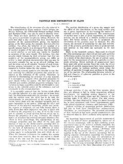
5 Adjustments are made within the operating software so that the equipment provides the calibration material diameter. The equipment provides a full size analysis, an example is provided in Figure and Section In Fig. Example size distribution Malvern Note, for descriptions of principles of operation see the recommended web sites. Fundamentals of Particle technology 7 order to simplify subsequent description and calculations it is usual to attempt to represent the full Particle size distribution by a single diameter. Unfortunately, there are many possibilities and the median, or x50, is commonly (and usually mistakenly) applied. This diameter is easily read off the cumulative distribution curve (see right). At this stage, the reader may well reflect on the best way to represent the Particle size data. There are a number of options to consider: which equivalent spherical diameter, which size analytical equipment and which statistical diameter (mean, median, mode)?

6 The most appropriate technique for the end use of the data should be used. For example, if the data is required to design a settling basin for effluent removal a sedimentation diameter is best. If the data is to be used in reaction engineering, or mass transfer calculations, then the equivalent spherical diameter by surface area per unit volume (or mass) is the most appropriate. In the latter case, it is the surface area that dictates the reactivity and is used in the equations for these subjects. However, it should be noted that the surface area exhibited to fluid flow is not, necessarily, the same as that exhibited to reactants in the gaseous phase. Catalyst particles often have a structure that provides internal surfaces for reaction. This will be discussed again in Chapter 7. Particle size functions One of the harder concepts to follow is that the Particle size function of the same powder depends upon the basis on which it is reported.

7 This is for similar reasons to the different values found in exercise An illustration of this is given in Figures and , and the data used to construct the curves is included. Firstly, it is a trivial matter to take the total number of particles and convert to a fractional amount in each size range (or grade). Hence, it is possible to plot the cumulative number of particles undersize against Particle size . Clearly all the particles are less than 51 m; hence, 100%, or as a fraction, are less than this size . At the next size increment boundary, 41 m, there are particles less than this size ; so, the cumulative number less than 41 m is , etc. Finally, there are no particles less than 1 m; hence, the cumulative number undersize is zero at this point. The above example covers a consideration of the number fraction of particles within size ranges, or grades (for example: 31 to 41 m).

8 It is quite common to want to consider the size distribution based upon mass rather than number. This can be achieved by conversion from the number distribution as follows. The mass of a single Particle is svxk 3 where kv is the volume shape coefficient. For spheres, the volume shape coefficient is /6; it is the factor that the diameter cubed must be multiplied by in order to give the volume of the shape. Hence, the mass of many particles within a size range will be fxks3v Fig. Example distribution 8 Particle characterisation where f is the number of particles in that size range. The mass fraction, within a size range and compared to the total mass of the distribution (mi), will be the mass in the size range in question divided by the mass of the entire distribution ; = =i3ii3iis3ivis3ivifxfxfxkfxkm ( ) Equation ( ) assumes that the volume shape coefficient and the solid density remain constant throughout all the size grades and, therefore, can be cancelled.

9 Also, in order to apply the equation we need to define a size to use for xi; this is usually the mid-point of the grade. Thus, in the size grade 31 to 41 m, the mid-point is 36 m, and it would be multiplied by the number of particles within the grade to give a value proportional to the mass in that grade. The constant of proportionality being the solid density multiplied by the volume shape factor. On consideration of equation ( ) it will become apparent that a mass based distribution will provide greater emphasis on the coarser particles than a number based one. This follows from the simple fact that one large Particle has much more mass than one small Particle : both represent a number distribution of one, but the distribution of mass is much greater in the larger Particle grade. Problem 2, page 18, covers the conversion of data from a number to a mass distribution .

10 On consideration of equation ( ) it should be apparent that a mass distribution is exactly the same as a volume distribution : to convert from volume to mass in each grade the true solids density is used, but to convert from mass in each grade to mass fraction the summation of the mass in each grade is divided into the component grade masses and the density will, in fact, cancel. Hence, the terms volume and mass distribution are used interchangeably. Mass and number distributions are frequently met within industry, but distributions by length and area also exist. In the latter case it may be by projected area (like looking down a microscope) or surface area; see page 5 for the equations of these for a sphere. The analogue expression for projected area to equation ( ) is = i2ii2ii2ipi2ipfxfxfxkfxk ( ) where kp is the projected area shape factor, /4 for spheres. In the construction of Figure the cumulative number undersize curve was considered.