Transcription of 21 Bootstrapping Regression Models - SAGE Publications …
1 21 BootstrappingRegressionModelsBootstrappi ngis a nonparametric approach to statistical inference that substitutes computationfor more traditional distributional assumptions and asymptotic offersa number of advantages: The bootstrap is quite general, although there are some cases in which it fails. Because it does not require distributional assumptions (such as normally distributed errors),the bootstrap can provide more accurate inferences when the data are not well behaved orwhen the sample size is small. It is possible to apply the bootstrap to statistics with sampling distributions that are difficultto derive, even asymptotically.
2 It is relatively simple to apply the bootstrap to complex data-collection plans (such asstratified and clustered samples). Bootstrapping BasicsMy principal aim is to explain how to bootstrap Regression Models (broadly construed to includegeneralized linear Models , etc.), but the topic is best introduced in a simpler context: Supposethat we draw an independent random sample from a large concreteness andsimplicity, imagine that we sample four working, married couples, determining in each case thehusband s and wife s income, as recorded in Table I will focus on the difference in incomesbetween husbands and wives, denoted asYifor theith want to estimate the mean difference in income between husbands and wives in the pop-ulation.
3 Please bear with me as I review some basic statistical theory: A point estimate of thispopulation mean difference is the sample mean,Y= Yin=6 3+5+34= statistical theory tells us that the standard deviation of the sampling distribution ofsample means is SD(Y)= / n, where is the population standard deviation we knew , and ifYwere normally distributed, then a 95% confidence interval for wouldbe =Y n1 The termbootstrapping, coined by Efron (1979), refers to using the sample to learn about the sampling distribution ofa statistic without reference to external assumptions as in pulling oneself up by one s bootstraps.
4 2In anindependent random sample, each element of the population can be selected more than once. In asimple randomsample, in contrast, once an element is selected into the sample, it is removed from the population, so that sampling isdone without replacement. When the population is very large in comparison to the sample (say, at least 10 times aslarge), the distinction between independent and simple random sampling becomes 21. Bootstrapping Regression ModelsTable Sample of Four Married Couples, ShowingHusbands and Wives Incomes in Thousands of DollarsObservationHusband s IncomeWife s IncomeDifference Yi12418621417 is the standard normal value with a probability of.
5 025 to the right. IfYisnotnormally distributed in the population, then this result applies asymptotically. Of course, theasymptotics are cold comfort whenn= a real application, we do not know . The standard estimator of isS= (Yi Y)2n 1from which the standard error of the mean ( , theestimatedstandard deviation ofY)isSE(Y)=S/ n. If the population is normally distributed, then we can take account of the added uncertaintyassociated with estimating the standard deviation of the mean by substituting the heavier-tailedt-distribution for the normal distribution, producing the 95% confidence interval =Y tn 1.
6 025S nHere,tn 1,.025is the critical value oftwithn 1 degrees of freedom and a right-tail probabilityof . the present case,S= , SE(Y)= 4= , andt3,.025= The 95%confidence interval for the population mean is thus = , equivalently, < < one would expect, this confidence interval which is based on only four observations isvery wide and includes 0. It is, unfortunately, hard to be sure that the population is reasonablyclose to normally distributed when we have such a small sample, and so thet-interval may not begins by using the distribution of data values in the sample (here,Y1=6,Y2= 3,Y3=5,Y4=3) toestimatethe distribution ofYin the is, we define therandom variableY with distribution53To say that a confidence interval is valid means that it has the stated coverage.
7 That is, a 95% confidence interval isvalid if it is constructed according to a procedure that encloses the population mean in 95% of alternative would be to resample from a distribution given by a nonparametric density estimate (see, , Silverman& Young, 1987). Typically, however, little if anything is gained by using a more complex estimate of the populationdistribution. Moreover, the simpler method explained here generalizes more readily to more complex situations in whichthe population is multivariate or not simply characterized by a asterisks onp ( ), E ,andV remind us that this probability distribution, expectation, and variance are conditionalon the specific sample in hand.
8 Were we to select another sample, the values ofY1,Y2,Y3,andY4, would change and along with them the probability distribution ofY , its expectation, and Bootstrapping Basics589y p (y ) thatE (Y )= ally y p(y )= (Y )= [y E (Y )]2p(y )= 1nS2 Thus, the expectation ofY is just the sample mean ofY, and the variance ofY is [except forthe factor(n 1)/n, which is trivial in larger samples] the sample variance next mimic sampling from the original population by treating the sample as if it werethe population, enumerating all possible samples of sizen=4 from the probability distributionofY . In the present case, eachbootstrap sampleselects four valueswith replacementfromamong the four values of the original sample.
9 There are, therefore, 44=256 different bootstrapsamples,6each selected with probability 1/256. A few of the 256 samples are shown in Table the four observations in each bootstrap sample are chosen with replacement, particularbootstrap samples usually have repeated observations from the original sample. Indeed, of theillustrative bootstrap samples shown in Table , only sample 100 doesnothave us denote thebth bootstrap sample7asy b=[Y b1,Y b2,Y b3,Y b4] , or more generally,y b=[Y b1,Y b2,.. ,Y bn] , whereb=1, 2,.. ,nn. For each such bootstrap sample, wecalculate the mean,Y b= ni=1Y binThe sampling distribution of the 256 bootstrap means is shown in Figure mean of the 256 bootstrap sample means is just the original sample mean,Y= Thestandard deviation of the bootstrap means isSD (Y )= nnb=1(Y b Y)2nn= divide here bynnrather than bynn 1 because the distribution of thenn=256 bootstrapsample means (Figure ) is known,notestimated.
10 The standard deviation of the bootstrap6 Many of the 256 samples have the same elements but in different order for example, [6, 3, 5, 3] and [3, 5, 6, 3]. Wecould enumerate the unique samples without respect to order and find the probability of each, but it is simpler to workwith the 256 orderings because each ordering has equal vector notation is unfamiliar, then think ofy bsimply as a list of the bootstrap observationsY bifor 21. Bootstrapping Regression ModelsTable Few of the 256 Bootstrap Samples for theData Set [6, 3, 5, 3], and the CorrespondingBootstrap Means,Y bBootstrap SamplebY b1Y b2Y b3Y b4Y 3 3563 35 36 is nearly equal to the usual standard error of the sample mean.