Transcription of 360-2008: Convergence Failures in Logistic Regression
1 1 Paper 360-2008 Convergence Failures in Logistic Regression Paul D. Allison, University of Pennsylvania, Philadelphia, PA ABSTRACT A frequent problem in estimating Logistic Regression models is a failure of the likelihood maximization algorithm to converge. In most cases, this failure is a consequence of data patterns known as complete or quasi-complete separation. For these patterns, the maximum likelihood estimates simply do not exist. In this paper, I examine how and why complete or quasi-complete separation occur, and the effects they produce in output from SAS procedures. I then describe and evaluate several possible solutions. INTRODUCTION Anyone with much practical experience using Logistic Regression will have occasionally encountered problems with Convergence .
2 Such problems are usually both puzzling and exasperating. Most researchers do not have a clue as to why certain models and certain data sets lead to Convergence difficulties. And for those who do understand the causes of the problem, it is often unclear whether and how the problem can be fixed. In this paper, I explain why numerical algorithms for maximum likelihood estimation of the Logistic Regression model sometimes fail to converge, and I consider a number possible solutions. I also look at how several SAS procedures handle the problem. This paper is a revised and updated version of Allison (2004). ML ESTIMATION OF THE Logistic Regression MODEL I begin with a review of the Logistic Regression model and maximum likelihood estimation its parameters.
3 For further details, see Allison (1999). For a sample of n cases (i=1,..,n), we have data on a dummy dependent variable yi (with values of 1 and 0) and a column vector of explanatory variables xi (including a 1 for the intercept term). The Logistic Regression model states that )exp(11)|1Pr(iiiy xx +== (1) where is a row vector of coefficients. Equivalently, the model may be written in logit form: iiiiiyy xxx= ==)|0Pr()|1Pr(ln. (2) Assuming that the n cases are independent, the log-likelihood function for this model is + =iiiiiy)]exp(1ln[)( xx l (3) The goal of maximum likelihood estimation is to find a set of values for that maximize this function.
4 One well-known approach to maximizing a function like this is to differentiate it with respect to , set the derivative equal to 0, and then solve the resulting set of equations. The first derivative of the log-likelihood is iiiiiiyy )( = xx l (4) whereiy , the predicted value of y, is given by )exp(11 iiy x +=. (5) The next step is to set the derivative equal to 0 and solve for : Statistics and Data AnalysisSASG lobalForum2008 2 0xx= iiiiiiyy (6) Because is a vector, (6) is actually a set of equations, one for each of the parameters to be estimated. These equations are identical to the normal equations for least-squares linear Regression , except that by (5) iy is a non-linear function of the xi s rather than a linear function.
5 For some models and data ( , saturated models), the equations in (6) can be explicitly solved for the ML estimator . For example, suppose there is a single dichotomous x variable, so that the data can be arrayed in a 2 2 table, with observed cell frequencies f11, f12, f21, and f22. Then the ML estimator of the coefficient of x is given by the logarithm of the cross-product ratio : =22212211ln ffff . (7) For most data and models, however, the equations in (6) have no explicit solution. In such cases, the equations must be solved by numerical methods, of which there are many. The most popular numerical method is the Newton-Raphson algorithm. Let )( Ube the vector of first derivatives of the log-likelihood with respect to and let )( Ibe the matrix of second derivatives.
6 That is, ) 1( ')() )()2iiiiiiiiiiiyyyy = = = = xx I( xx U( ll (8) The vector of first derivatives )( Uis called the gradient while the matrix of second derivatives )( Iis called the Hessian. The Newton-Raphson algorithm is then )()(11jjjj U I + = (9) where I-1 is the inverse of I. To operationalize this algorithm, a set of starting values 0 is required. Choice of starting values is not critical; usually, setting 0 = 0 works fine. The starting values are substituted into the right-hand side of (9), which yields the result for the first iteration, 1.
7 These values are then substituted back into the right hand side, the first and second derivatives are recomputed, and the result is 2 . The process is repeated until the maximum change in each parameter estimate from one iteration to the next is less than some criterion, at which point we say that the algorithm has converged. Once we have the results of the final iteration, , a byproduct of the Newton-Raphson algorithm is an estimate of the covariance matrix of the coefficients, which is just ) (1 I . Estimates of the standard errors of the coefficients are obtained by taking the square roots of the main diagonal elements of this matrix. WHAT CAN GO WRONG? A common problem in maximizing a function is the presence of local maxima.
8 Fortunately, such problems cannot occur with Logistic Regression because the log-likelihood is globally concave, meaning that the function can have at most one maximum (Amemiya 1985). Unfortunately, there are many situations in which the likelihood function has no maximum, in which case we say that the maximum likelihood estimate does not exist. Consider the set of data on 10 observations in Table 1. Statistics and Data AnalysisSASG lobalForum2008 3 Table 1. Data Exhibiting Complete Separation. x y -5 0 -4 0 -3 0 -2 0 -1 0 1 1 2 1 3 1 4 1 5 1 For these data, it can be shown that the ML estimate of the intercept is 0.
9 Figure 1 shows a graph of the log-likelihood as a function of the slope beta . loglike-7-6-5-4-3-2-10bet a012345 Figure 1. Log-likelihood as a function of the slope under complete separation It is apparent that, although the log-likelihood is bounded above by 0, it does not reach a maximum as beta increases. We can make the log-likelihood as close to 0 as we choose by making beta sufficiently large. Hence, there is no maximum likelihood estimate. This is an example of a problem known as complete separation (Albert and Anderson 1984), which occurs whenever there exists some vector of coefficients b such that yi = 1 whenever bxi > 0 and yi = 0 whenever bxi 0. In other words, complete separation occurs whenever a linear function of x can generate perfect predictions of y.
10 For our hypothetical data set, a simple linear function that satisfies this property is 0 + 1(x). That is, when x is greater than 0, y=1, and when x is less than or equal to 0, y=0. A related problem is known as quasi-complete separation. This occurs when (a) there exists some coefficient vector b such that bxi 0 whenever yi = 1, and bxi 0 whenever yi = 0, and equality holds for at least one case in each category of the dependent variable. Table 2 displays a data set that satisfies this condition. Statistics and Data AnalysisSASG lobalForum2008 4 Table 2. Data Exhibiting Quasi-Complete Separation. x y -5 0 -4 0 -3 0 -2 0 -1 0 0 0 0 1 1 1 2 1 3 1 4 1 5 1 What distinguishes this data set from the previous one is that there are two additional observations, each with x values of 0 but having different values of y.