Transcription of 366-2008: The Use of Propensity Scores and Instrumental ...
1 1 Paper 366-2008 The Use of Propensity Scores and Instrumental variable methods to Adjust For Treatment Selection Bias R. Scott Leslie, MedImpact Healthcare Systems, Inc., San Diego, CA Hassan Ghomrawi, MedImpact Healthcare Systems, Inc., San Diego, CA ABSTRACT Observational studies that lack randomization of subjects into treatment groups must address selection bias to properly estimate the effect of treatment. This paper explores a Propensity scoring (PS) method and Instrumental variable (IV) method of controlling for treatment selection bias. Included is a discussion of the methods , the advantages and disadvantages of the two methods as well as a comparison of results when applied to a study that evaluates the effect of therapy regimen on medication adherence. The LOGISTIC procedure is used to create Propensity Scores and the QLIM procedure in SAS/ETS is used to conduct Instrumental variable analysis.
2 INTRODUCTION Among the strengths of observational studies is the ability to estimate treatment effect in real world conditions. On the contrary, a limitation of observational studies is the lack of treatment assignment. Non randomized groups usually differ in observed and unobserved characteristics resulting in differential selection into treatment groups causing selection bias when evaluating the effect of treatment. Regression adjustment, matching, and stratification using Propensity Scores are widely used techniques to compare groups, usually comparing a treatment group to a non treatment group. Instrumental variable analysis is the standard method used to control for selection bias in economic circles. The purpose of this paper is to explain and contrast methods using an example of diabetic members taking two different therapy regimens.
3 Treatment groups were compared by medication adherence defined as the proportion of days of medication coverage over a 1-year period. DESCRIPTION OF STUDY In this study, we identified 19,433 patients using oral antidiabetic therapy from a large pharmacy claims database. Patients were categorized into two drug treatment groups, A and B, with the main objective of comparing compliance and adherence rates. Compliance was measured as the proportion of days a medication was supplied over a 180 day period. Adherent patients were identified as those reaching a threshold of 80% compliance. Selection bias is believed to be a factor as the two drug treatment groups differ in patient tolerance, adverse events, and side effects which possibly influence compliance to each drug. Other variables controlled for in the analyses include demographic variables (age, gender) and previous medication use/patterns that were measured in a 6 month baseline period prior to treatment.
4 Previous medication use was recorded by the use of specific cardiovascular, asthma, and antidepressant medications and previous medication pattern use was measured by refill patterns of maintenance type medications. Table 1 describes the two treatment groups. PROC GLM was used to compare groups. Few covariates significantly differed. Table 1. Unadjusted Demographic and Baseline Measures UNADJUSTED VALUES Drug A Drug B Member Count 9,129 10,304 Mean Age SD Female % HMO % Mean # of Drugs Utilized SD Maintenance Medication Refill * % Prior Use * Naive/Naive % Experienced/Experienced % Naive/Experienced User % Statistics and Data AnalysisSASG lobalForum2008 2 UNADJUSTED VALUES Drug A Drug B Sulfonylurea
5 * % Hypertension % Lipid Irregularity % Pain Management * % Antidepressant % Asthma % * p < .05 Below is a distribution of the outcomes for the two treatment groups. Mean compliance for drug A and drug B was and , respectively. Although statistically different (p = ), the difference between groups is less than 1 percentage point and the distributions are very similar.
6 Since compliance was measured as the proportion of days the medication was supplied over the 180 day period, the maximum allowable value was 1. 02. 55. 07. 510. 012. 515. 0 PercentDrugA- 0. 165 - 0. 0450. 0750. 1950. 3150. 4350. 5550. 6750. 7950. 9151. 0351. 15502. 55. 07. 510. 012. 515. 0 PercentDrugBPr opor t i on of Days Cover ed Propensity score ANALYSIS The Propensity score is the conditional probability of each patient receiving a particular treatment based on pre- treatment variables. Using the LOGISTIC procedure, Propensity Scores were calculated based on the covariates listed in Table 1. The objective was to balance the treatment groups so to reduce bias of treatment selection and obtain better idea of treatment effect on the outcome of compliance. The logit function is specified in the LINK option to fit the binary logit model and the RSQUARE option assesses the amount of variation explained by the independent variables.
7 The Propensity score is output to data set named psdataset . The predicted probabilities are output to a variable named ps . Statistics and Data AnalysisSASG lobalForum2008 3 proc logistic data = wuss; class preuser; model tx (event=first) = age female pre_drug_cnt_subset preuser maintrefillratio copay_idxdrug pre_sulf _0106 _0109 _0112 _0113 _0149 /link=logit rsquare; output out=psdataset pred=ps; format preuser $preuser.; run; After creating the Propensity Scores , an evaluation of the distributions by treatment group checks for sizeable overlap among the groups demonstrating that the groups are comparable. 02468101214 PercentDrugA0. 33 0. 35 0. 37 0. 39 0. 41 0. 43 0. 45 0. 47 0. 49 0. 51 0. 53 0. 55 0. 57 0. 59 0. 61 0. 6302468101214 PercentDrugBEs t i mated Probability A Propensity score weight, also referred to as the inverse probability of treatment weight (IPTW), is calculated as the inverse of the Propensity score .
8 The treatment selection model above modeled the Propensity to receive drug a. For those patients receiving drug b, the Propensity score would be 1- ps and the Propensity score weight would be the inverse of 1-ps. data psdataset; set psdataset; if druga=1 then ps_weight=1/ps;else ps_weight=1/(1-ps); run; Statistics and Data AnalysisSASG lobalForum2008 4 Propensity score WEIGHTED OUTCOME MODEL Next, a Propensity score -weighted linear regression model was fitted to compare drug treatment on the outcome of compliance while controlling for other covariates. The GLM procedure is used to takes advantage of continuous and categorical covariates. The LSMEANS statement computes the least-squares means for the treatment variable allowing for multiple comparisons The ADJUST=TUKEY option uses the Tukey-Kramer method to adjust the lease-square means and the PDIFF and CL options give the p values and corresponding confidence intervals for the differences in the least-squares means.
9 Proc glm data=psdataset; class tx preuser; model p_dayscovered = tx age female copay_idxdrug pre_drug_cnt_subset preuser maintrefillratio pre_sulf _0106 _0109 _0112 _0113 _0149 /solution; lsmeans tx/OM ADJUST=TUKEY PDIFF CL; weight ps_weight; format preuser $preuser.; quit; Results of the model above showed no difference between treatment groups (p = ). Compared to the unadjusted compliance means (a model with compliance as the dependent variable and drug treatment as the only independent variable ) shows the effect of controlling for confounding. The increase in compliance from the unadjusted means ( and ) to the adjusted means ( and ) was probably due to the large number of patients with prior use of the drug. These patients had higher compliance values than those new to therapy and therefore when this variable is placed in the model as a covariate the mean compliance values rise.
10 Table 2. Mean Compliance by Treatment: Unadjusted vs. PS Adjusted Models Model Treatment Compliance Outcome 95% Confidence Limits Unadjusted Model P = Drug A Drug B Propensity score Adjusted Model P = Drug A
![Index [www.fandept.com]](/cache/preview/8/2/1/7/a/e/c/d/thumb-8217aecd553b7e6a7bea5aba32403881.jpg)