Transcription of 427-2013: Creating and Customizing the Kaplan-Meier ...
1 Paper 427-2013 Creating and Customizing the Kaplan-Meier Survival Plot in PROC LIFETESTW arren F. Kuhfeld and Ying So, SAS Institute you are a medical, pharmaceutical, or life sciences researcher, you have probably analyzed time-to-event data (survivaldata). One of several survival analysis procedures that SAS/STAT provides, the LIFETEST procedure computesKaplan- meier estimates of the survivor functions and compares survival curves between groups of patients. You can usethe Kaplan-Meier plot to display the number of subjects at risk, confidence limits, equal-precision bands, Hall-Wellnerbands, and homogeneity testp-value. You can control the contents of the survival plot by specifying procedure optionswith PROC LIFETEST. When the procedure options are insufficient, you can modify the graph templates with SAS paper provides examples of survival plot modifications using procedure options, graph template modifications usingmacros, and style template that measure lifetime or the length of time until the occurrence of an event are calledsurvivaldata.
2 Survival dataare often medical data; examples include the survival time for heart transplant or cancer patients. Survival time is ameasure of the duration of time until a specified event (such as relapse or death) occurs. Survival data consist of survivaltime and possibly a set of independent variables thought to be associated with the survival time variable. The systemthat gives rise to the event of interest can be biological (as for most medical data) or physical (as for engineering data).Survival analysis estimates the underlying distribution of the survival time variable and assesses the dependence of thesurvival time variable on the independent data analysis methods are not appropriate for survival data. Survival times are generally positively skewed,and it is not reasonable to assume that data of this type have a normal distribution. Furthermore, survival times are oftencensored. The survival time of an individual is right censored when the event of interest has not been observed for thatindividual.
3 For example, a patient who is recruited for a clinical trial drops out of the trial or the event is not observedwhen the period of data collection ends. In either case, the observed time is less than the true survival time. Analysis ofsurvival data must take censoring into account and correctly use both the censored observations and the LIFETEST procedure in SAS/STAT is a nonparametric procedure for analyzing survival data. You can use PROCLIFETEST to compute the Kaplan-Meier (1958) curve, which is a nonparametric maximum likelihood estimate of thesurvivor function. You can display the Kaplan-Meier plot that contains step functions representing the kaplan -Meiercurves of different samples. You can also use PROC LIFETEST to compare the survivor functions of different samplesby the log-rank data that are used in this paper come from 137 bone marrow transplant patients in a study byKlein and Moeschberger(1997) and are available in the BMT data set in the Sashelp library.
4 At the time of transplant, each patient is classifiedin one of three risk categories: ALL (acute lymphoblastic leukemia), AML (acute myelocytic leukemia) Low-Risk,and AML High-Risk. The endpoint of interest is the disease-free survival time, which is the time in days until death,relapse, or the end of the study. The variableGrouprepresents the patient s risk category, the variableTrepresents thedisease-free survival time, and the variableStatusis the censoring indicator. A status of 1 indicates an event time, and astatus of 0 indicates a censored examples use the release of SAS software from 2012. Three types of examples are provided: specifyingprocedure options, modifying graph templates, and modifying style THE SURVIVAL PLOT BY SPECIFYING PROCEDURE OPTIONSThis section provides a series of examples that use ODS Graphics and the PLOTS= option in the PROC LIFETEST statement to control the appearance of the survival plot.
5 You can use the following statements to enable ODS Graphicsand run PROC LIFETEST:ods graphics on;ods select survivalplot(persist) failureplot(persist);proc lifetest data= ;time T*Status(0);strata Group;run;The results are displayed in Figure 1. ODS Graphics is enabled for this step and all subsequent steps until ODS Graphicsis disabled. ODS Graphics remains enabled throughout the examples in this paper. The ODS SELECT statementpersistently selects just the survival and failure time plot for this and subsequent steps. Each analysis produces only oneof these two plots. You specify in the TIME statement that the disease-free survival time is recorded in the can further specify that the variableStatusindicates censoring and 0 indicates a censored time. Separate survivorfunctions are compared for each of the groups in theGroupvariable, which you specify in the STRATA statement. Thegraph inFigure 1consists of three step functions, one for each of the three groups of patients.
6 The graph shows thatpatients in the AML Low-Risk group have longer disease-free survival than patients in the ALL and AML and Data AnalysisSASG lobalForum2013 Figure 1: Default Kaplan-Meier PlotFigure 2: One of Three Individual PlotsFigure 3: Individual Plots Displayed in a PanelFigure 4: Confidence Bands and Homogeneity TestThe PLOTS= option enables you to control some details of the graphs. You can use it to request nondefault graphs andspecify options for all graphs. For example, you can use the STRATA=INDIVIDUAL option to request individual survivalplots. By default, the STRATA=OVERLAY option produces the graph of overlaid step functions displayed inFigure 1. Youcan run the same analysis but request the results in three separate graphs, one per patient group, as follows:proc lifetest data= plots=survival(strata=individual);time T*Status(0);strata Group;run;The first of the three survival plots is displayed in Figure 2.
7 In the interest of space, the other graphs are not can use the STRATA=PANEL option as follows to display the results in separate panels of a single graphical display:proc lifetest data= plots=survival(strata=panel);time T*Status(0);strata Group;run;The results are displayed in Figure rest of this paper discusses overlaid plots such as the one displayed inFigure 1. You can use the followingstatements to add Hall-Wellner confidence bands (Hall and Wellner 1980) toFigure 1and display thep-value from a testthat the strata are homogeneous:proc lifetest data= plots=survival(cb=hw test);time T*Status(0);strata Group;run;The results are displayed inFigure 4. The Hall-Wellner confidence bands extend to the last event. The smallp-valuesupports rejecting the hypothesis that the groups are and Data AnalysisSASG lobalForum2013 Figure 5: At-Risk Table Inside the PlotFigure 6: At-Risk Table with LabelsYou can add the at-risk table as follows:proc lifetest data= plots=survival(cb=hw test atrisk);time T*Status(0);strata Group;run;The results are displayed in Figure 5.
8 By default, the at-risk table is displayed inside the body of the graph . For thesedata, the default survival times are 0, 1000, 2000, and 3000. You will see how to specify other values in subsequentexamples. This table shows the number of patients who are at risk for each group for each of the different group labels for the at-risk table are group numbers, and these numbers appear in the legend. Numbers are usedrather than the actual labels because the length of the longest label (13) is greater than the default set by the maximumlabel length option (MAXLEN=12). You can display labels rather than the group numbers by specifying a MAXLEN=value equal to the maximum group label length as follows:proc lifetest data= plots=survival(cb=hw test atrisk(maxlen=13));time T*Status(0);strata Group;run;The results are displayed in Figure 6. The legend entries and the order of the rows in the at-risk table correspond to thesort order of the values of theGroupvariable.
9 You can change the order by first mapping each value to a new valuein the desired order, and then running the analysis by using a FORMAT statement to provide the original values. Thefollowing steps illustrate:proc format;invalue bmtnum 'ALL' = 1 'AML-Low Risk' = 2 'AML-High Risk' = 3;value bmtfmt 1 = 'ALL' 2 = 'AML-Low Risk' 3 = 'AML-High Risk';run;data BMT(drop=g);set (rename=(group=g));Group = input(g, bmtnum.);run;proc lifetest data=BMT plots=survival(cl test atrisk(maxlen=13));time T*Status(0);strata Group / order=internal;format group bmtfmt.;run;The PROC FORMAT step has two statements. The INVALUE statement creates an informat that maps the values ofthe originalGroupvariable into integers that have the right order. The VALUE statement creates a format that mapsthe integers back to the original values. The informat is used in the DATA step to create a new specify the ORDER=INTERNAL option in the STRATA statement of PROC LIFETEST step to sort theGroupvaluesbased on internal order (the order specified by the integers, which are the internal unformatted values).
10 The FORMAT statement is used to assign the BMTFMT format to theGroupvariable so that the actual risk groups are displayed inthe analysis. This example also illustrates the use of the CL option, which displays pointwise confidence limits for thesurvival curve (instead of the Hall-Wellner confidence bands). The results are displayed inFigure and Data AnalysisSASG lobalForum2013 Figure 7: Controlling Legend OrderFigure 8: Failure PlotFigure 9: Censored Values Not DisplayedFigure 10: At-Risk Table Outside the PlotAll the discussion up to this point has been about survival plots. You can instead plot failure probabilities by using thePLOTS=SURVIVAL(FAILURE) option as follows:proc lifetest data=BMT plots=survival(cb=hw failure test atrisk(maxlen=13));time T*Status(0);strata Group / order=internal;format group bmtfmt.;run;The results are displayed in Figure can use the PLOTS=SURVIVAL(NOCENSOR) option to suppress the display of censored observations as follows:proc lifetest data=BMT plots=survival(nocensor test atrisk(maxlen=13));time T*Status(0);strata Group / order=internal;format group bmtfmt.