A Beginner’s Guide to Materials Studio and DFT ...

1 A beginner 's Guide to Materials Studio and DFT Calculations with Castep P. Hasnip September 18, 2007. Materials Studio collects all of its files into Projects . We'll start by creating a new project. 1. Now we've got a blank project, and we want to define a simulation cell to perform a Castep calculation on. First we add a 3D Atomistic document . 2. 3. We're going to start by simulating an eight atom silicon FCC cell, so rename the file ac- cordingly. First we'll create the unit cell. 4. 5. The default is space group P1, no symme- try. Silicon has the diamond structure (space group FD3M). By telling Materials Studio this symmetry it will automatically apply it to the atoms, thus generating atoms at the symmetry points. 6. Now to add the lattice constant click on the Lattice tab near the top of the Build Crystal window. Since FD3M is cubic (FCC). Materials Studio knows only a has to be set, and the angles and other lattice constants are greyed-out.

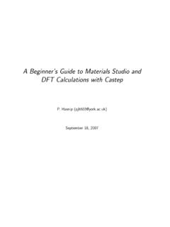
2 Enter , and then click on Build . 7. Now we'll add a single silicon 8. Add a silicon atom at the origin, by chang- ing the element from its default and click- ing Add . By default the co-ordinates are in fractionals, but you can change this on the Options tab. 9. Since we'd already told Materials Studio what the symmetry of the crystal was, our single sil- icon atom is replicated at each symmetry site and we now have a shiny new eight-atom sili- con unit cell. You can rotate the view by holding down the left or right mouse button and dragging, or move it by holding down the middle button. Use the mouse wheel, or both the left and right buttons simultaneously, to zoom in and out. 10. By default the atoms are shown as little crosses with lines for bonds, and silicon atoms are coloured brownish orange. You can always change this if you don't like it. The bonds are just guesses made by Materials Studio based on the ele- ment's typical bond-lengths.

3 We're now ready to run Castep to find the groundstate charge density. Click on the Castep icon, which is a set of three wavy lines (to rep- resent plane-waves), and select calculation . 11. Materials Studio offers a high-level interface to Castep, with cut-off energy, k-point sampling, convergence tolerances etc. all set by the sin- gle setting Quality . We'll look at how to specify these things later, but for now we'll just do a very quick, rough calculation of the groundstate energy and density of our cell. Make sure the task is Energy , and select Coarse for quality, and LDA for the XC. functional. 12. If you want to run your calculations on La- gavulin (or anywhere else you have Castep avail- able) then you'll want to click Files in the Castep window. Simply select Save Files to save the cell and param files. By default these are written to a folder in My Documents called Materi- als Studio Projects but be warned cell files are hidden files, and you won't be able to see them unless you tell Windows you want to view Hidden and System Files for that folder.

4 13. If you want to run Castep on the PC you're us- ing, you just need to click Run on the Castep window. You should see this window appear: Materials Studio is telling you that your system isn't actually the primitive unit cell, and it's offering to convert it to the primitive cell for you. For now choose No . Castep runs via a Gateway , which might be on your local computer or on a remote ma- chine. This Gateway handles Materials Stu- dio's requests to run calculations and copies the files to and from the Castep Server . 14. Since the Gateway is actually a modified web server it is sensible to enforce some security measures. If your Gateway is password-protected (recom- mended), you'll need to enter your Gateway username and password (which are not neces- sarily the same as your Windows ones). 15. When the Castep job is running you will see its job ID and other details appear in the job ex- plorer window.

5 You can check its status from here, although our crude silicon calculation is so quick you probably won't have time now. 16. Castep reports back when it is finished, and Materials Studio copies the results of the cal- culation back. The .castep file is opened au- tomatically so you can see what happened in the calculation . The main text output file from castep is dis- played in Materials Studio . It starts with a wel- come banner, then a summary of the parame- ters and cell that were used for the calculation . 17. After that, there is a summary of the elec- tronic energy minimisation which shows the it- erations Castep performed trying to find the groundstate density that was consistent with the Kohn-Sham potential. This is the so-called self-consistent field or SCF condition, and each line is tagged with SCF so you can find them easily. ---------------------------------------- -------------------------------- <-- SCF.

6 SCF loop Energy Fermi Energy gain Timer <-- SCF. energy per atom (sec) <-- SCF. ---------------------------------------- -------------------------------- <-- SCF. Initial +002 +001 <-- SCF. Warning: There are no empty bands for at least one kpoint and spin; this may slow the convergence and/or lead to an inaccurate groundstate. If this warning persists, you should consider increasing nextra_bands and/or reducing smearing_width in the param file. Recommend using nextra_bands of 7 to 15. 1 +002 +001 +002 <-- SCF. 2 +002 +000 +001 <-- SCF. 3 +002 +000 +000 <-- SCF. 4 +002 +000 <-- SCF. 5 +002 +000 <-- SCF. 6 +002 +000 <-- SCF. 7 +002 +000 <-- SCF. 8 +002 +000 <-- SCF. ---------------------------------------- -------------------------------- <-- SCF. Final energy, E = eV. Final free energy (E-TS) = eV. (energies not corrected for finite basis set). NB est.

7 0K energy ( ) = eV. 18. We'll look at this output in more detail later. For now just note that the energy converges fairly rapidly to about , but that the energy is sometimes higher than this and some- times lower. Let's have a look at the calculated groundstate charge density. 19. The Castep Analysis window lets you look at various properties you might have calculated during the Castep job. Select Electron den- sity . Notice there's a Save button which lets you write the density out to a text file so you can analyse it with another program. We don't need this now, so just click on Import . 20. WARNING: amongst the properties listed here are Band structure and Density of states . If you select one of these from an energy cal- culation, Materials Studio will plot the band structure/DOS, but it takes the eigenvalues and k-points from the SCF calculation , not a proper band structure or DOS calculation .

8 21. By default an isosurface of the charge density is overlaid on your simulation cell. 22. To change the isosurface Materials Studio is plotting, you need to change the Display style . Either use the right mouse button when the cursor is over the simulation cell, or use the drop-down menus: Notice that this is also the place you need to come to if you want to change the atom colour- ing or representation ( from crosses and lines to ball-and-stick). 23. 24. Try changing the value of the isosurface your plotting, to see where the charge density is greatest and least. 25. Hopefully you've now got the hang of the basic interface. Go back to your simulation system and open up the Castep window again. This time select the Electronic tab. 26. This tab has a little more detail, and actually tells you what cut-off energy and k-point grid Castep will use for the given settings.

9 Never- theless we usually want finer control than this, so click on More . 27. Now at last we have four tabs that let us set some of the convergence parameters directly. 28. Basis Allows you to set a cut-off energy, as well as control the finite basis set correction. SCF. Sets the convergence tolerance for the ground- state electronic energy minimisation, as well as details of the algorithm used. k-points Controls the Brillouin zone sampling directly. You can either specify a grid, or a desired separation between k-points. Potentials Allows you to change the pseudopotentials used for the elements in your system. In fact if you double-click on your param file in the project window you can edit it directly, but we'll restrict ourselves to using the GUI for now. 29. Before we continue, here's a quick recap of the basic approximations we use when performing practical DFT calculations: Exchange-correlation (XC) Functional - we don't know the ex- act density functional, so we have to approximate it.

10 There are two common approximations: LDA - the Local Density Approximation assumes the XC at any point is the same as that of a homogeneous electron gas with the same density. PBE - this is a Generalised Gradient Approximation (GGA). and includes some of the effects of the gradient of the den- sity. You might think PBE is always better than LDA, but that's not true, both are approximations. You should try each one before deciding which is appropriate to your research project. Basis set - the wavefunction is represented by an expansion in a plane-wave basis. In theory the basis set required is infinite, but since the energy converges rapidly with basis set size we can safely truncate the expansion. The size of the basis set is controlled by the cut-off energy. Brillouin zone sampling - calculating the energy terms requires us to integrate quantities over the whole of the first Brillouin zone.