Transcription of A Tutorial on Bayesian Optimization of Expensive Cost ...
1 A Tutorial on Bayesian Optimization ofExpensive Cost Functions, with Application toActive User Modeling and HierarchicalReinforcement LearningEric Brochu, Vlad M. Cora and Nando de FreitasDecember 14, 2010 AbstractWe present a Tutorial on Bayesian Optimization , a method of findingthe maximum of Expensive cost functions. Bayesian Optimization employsthe Bayesian technique of setting a prior over the objective function andcombining it with evidence to get a posterior function. This permits autility-based selection of the next observation to make on the objectivefunction, which must take into account both exploration (sampling fromareas of high uncertainty) and exploitation (sampling areas likely to offerimprovement over the current best observation). We also present twodetailed extensions of Bayesian Optimization , with experiments activeuser modelling with preferences, and hierarchical reinforcement learning and a discussion of the pros and cons of Bayesian Optimization based onour IntroductionAn enormous body of scientific literature has been devoted to the problem ofoptimizing a nonlinear functionf(x) over a compact setA.
2 In the realm ofoptimization, this problem is formulated concisely as follows:maxx A Rdf(x)One typically assumes that theobjectivefunctionf(x) has a known mathe-matical representation, is convex, or is at least cheap to evaluate. Despite theinfluence of classical Optimization on machine learning, many learning problemsdo not conform to these strong assumptions. Often, evaluating the objectivefunction is Expensive or even impossible, and the derivatives and convexity prop-erties are many realistic sequential decision making problems, for example, one canonly hope to obtain an estimate of the objective function by simulating fu-ture scenarios. Whether one adopts simple Monte Carlo simulation or adaptive1 [ ] 12 Dec 2010schemes, as proposed in the fields of planning and reinforcement learning, theprocess of simulation is invariably Expensive .
3 Moreover, in some applications,drawing samplesf(x) from the function corresponds to Expensive processes:drug trials, destructive tests or financial investments. In active user modeling,xrepresents attributes of a user query, andf(x) requires a response from thehuman. Computers must ask the right questions and the number of questionsmust be kept to a minimum so as to avoid annoying the An Introduction to Bayesian OptimizationBayesian Optimization is a powerful strategy for finding the extrema of objectivefunctions that are Expensive to evaluate. It is applicable in situations where onedoes not have a closed-form expression for the objective function, but where onecan obtain observations (possibly noisy) of this function at sampled values. Itis particularly useful when these evaluations are costly, when one does not haveaccess to derivatives, or when the problem at hand is Optimization techniques are some of the most efficient approachesin terms of the number of function evaluations required (see, [Mo ckus, 1994,Joneset al.)]
4 , 1998, Streltsov and Vakili, 1999, Jones, 2001, Sasena, 2002]). Muchof the efficiency stems from the ability of Bayesian Optimization to incorporateprior belief about the problem to help direct the sampling, and to trade offexploration and exploitation of the search space. It is calledBayesianbecauseit uses the famous Bayes theorem , which states (simplifying somewhat) thattheposteriorprobability of a model (or theory, or hypothesis)Mgiven evi-dence (or data, or observations)Eis proportional to thelikelihoodofEgivenMmultiplied by thepriorprobability ofM:P(M|E) P(E|M)P(M).Inside this simple equation is the key to optimizing the objective function. InBayesian Optimization , thepriorrepresents our belief about the space of possibleobjective functions. Although the cost function is unknown, it is reasonable toassume that there exists prior knowledge about some of its properties, such assmoothness, and this makes some possible objective functions more plausiblethan s definexias theith sample, andf(xi) as the observation of the objectivefunction atxi.
5 As we accumulate observations1D1:t={x1:t,f(x1:t)}, the priordistribution is combined with the likelihood functionP(D1:t|f). Essentially,given what we think we know about the prior, how likely is the data we haveseen? If our prior belief is that the objective function is very smooth and noise-free, data with high variance or oscillations should be considered less likely thandata that barely deviate from the mean. Now, we can combine these to obtainour posterior distribution:P(f|D1:t) P(D1:t|f)P(f).1 Here we use subscripts to denote sequences of data, :t={y1, .. , yt}.2acquisition maxacquisition function (u( ))observation (x)objective fn (f( ))t = 2new observation (xt)t = 3posterior mean ( ( ))posterior uncertainty( ( ) ( ))t = 4 Figure 1:An example of using Bayesian Optimization on a toy 1D design figures show a Gaussian process (GP) approximation of the objective function overfour iterations of sampled values of the objective function.
6 The figure also shows theacquisition function in the lower shaded plots. The acquisition is high where the GPpredicts a high objective (exploitation) and where the prediction uncertainty is high(exploration) areas with both attributes are sampled first. Note that the area on thefar left remains unsampled, as while it has high uncertainty, it is (correctly) predictedto offer little improvement over the highest posterior captures our updated beliefs about the unknown objective func-tion. One may also interpret this step of Bayesian Optimization as estimatingthe objective function with asurrogate function(also called aresponse sur-face), described formally in with the posterior mean function of a sample efficiently, Bayesian Optimization uses an acquisition function todetermine the next locationxt+1 Ato sample.
7 The decision represents anautomatic trade-off between exploration (where the objective function is veryuncertain) and exploitation (trying values ofxwhere the objective function isexpected to be high). This Optimization technique has the nice property that itaims to minimize the number of objective function evaluations. Moreover, it islikely to do well even in settings where the objective function has multiple 1 shows a typical run of Bayesian Optimization on a 1D Optimization starts with two points. At each iteration, the acquisitionfunction is maximized to determine where next to sample from the objectivefunction the acquisition function takes into account the mean and variance ofthe predictions over the space to model the utility of sampling. The objectiveis then sampled at the argmax of the acquisition function, the Gaussian processis updated and the process is repeated.
8 +One may also interpret this stepof Bayesian Optimization as estimating the objective function with asurrogatefunction(also called aresponse surface), described formally in with theposterior mean function of a Gaussian OverviewIn 2, we give an overview of the Bayesian Optimization approach and its formally present Bayesian Optimization with Gaussian process priors ( )and describe covariance functions ( ), acquisition functions ( ) and the roleof Gaussian noise ( ). In , we cover the history of Bayesian Optimization ,and the related fields of kriging, GP experimental design and GP active second part of the Tutorial builds on the basic Bayesian optimizationmodel. In 3 and 4 we discuss extensions to Bayesian Optimization for activeuser modelling in preference galleries, and hierarchical control problems, respec-tively.
9 Finally, we end the Tutorial with a brief discussion of the pros and consof Bayesian Optimization in The Bayesian Optimization ApproachOptimization is a broad and fundamental field of mathematics. In order toharness it to our ends, we need to narrow it down by defining the conditions weare concerned first restriction is to simply specify that the form of the problem weare concerned with ismaximization, rather than the more common form ofminimization. The maximization of a real-valued functionx?= argmaxxf(x)can be regarded as the minimization of the transformed functiong(x) = f(x).We also assume that the objective isLipschitz-continuous. That is, thereexists some constantC, such that for allx1,x2 A: f(x1) f(x2) C x1 x2 ,thoughCmay be (and typically is) can narrow the problem down further by defining it as one ofglobal,rather thanlocaloptimization.
10 In local maximization problems, we need onlyfind a pointx(?)such thatf(x(?)) f(x), x(?) x < .4If f(x) is convex, then any local maximum is also a global maximum. However,in our Optimization problems, we cannot assume that the negative objectivefunction is convex. Itmightbe the case, but we have no way of knowing beforewe begin is common in global Optimization , and true for our problem, that the ob-jective is ablack boxfunction: we do not have an expression of the objectivefunction that we can analyze, and we do not know its derivatives. Evaluatingthe function is restricted to querying at a pointxand getting a (possibly noisy)response. Black box Optimization also typically requires that all dimensionshave bounds on the search space. In our case, we can safely make the sim-plifying assumption these bounds are all axis-aligned, so the search space is ahyperrectangle of number of approaches exist for this kind of global Optimization and havebeen well-studied in the literature ( , [T orn and Zilinskas, 1989, Mongeauet al.)]
![arXiv:1301.3781v3 [cs.CL] 7 Sep 2013](/cache/preview/4/d/5/0/4/3/4/0/thumb-4d504340120163c0bdf3f4678d8d217f.jpg)


![arXiv:0706.3639v1 [cs.AI] 25 Jun 2007](/cache/preview/4/1/3/9/3/1/4/b/thumb-4139314b93ef86b7b4c2d05ebcc88e46.jpg)
![@google.com arXiv:1609.03499v2 [cs.SD] 19 Sep 2016](/cache/preview/c/3/4/9/4/6/9/b/thumb-c349469b499107d21e221f2ac908f8b2.jpg)