Transcription of Abbr. Title Definition - SAS
1 1 Paper 079-31 Comparison of data preparation Methods for Use in Model Development with SAS Enterprise Miner By Charles Manahan, Ph. D. Cingular Wireless, LLC. Atlanta, GA ABSTRACT: SAS Enterprise Miner is a powerful tool for model development. By providing a GUI interface, drag and drop model evaluation, automatic record keeping of multiple scenarios, and scoring code generation, it saves a great deal of time over the traditional method using SAS STAT with the various regression PROCs. However, as most people who have developed predictive regression or other behavioral models are aware, the bulk of the time spent in developing models isn t in the final production of the regression coefficients, but in variable selection and preparing the input variables ( clustering levels, imputing missing values, etc.). Enterprise Miner has a module for variable selection and level condensation which is easy to use, but how well does this module compare with some traditional methods of variable selection?
2 Several models were developed in Enterprise Miner in parallel using traditional methods for data preparation vs the Enterprise Miner variable selection module. The results were then compared in Enterprise Miner to evaluate various data preparation methods. This is an intermediate level presentation and the audience should have knowledge of base SAS and conceptual knowledge of model evaluation, regression, and variable selection techniques. The audience should also have some familiarity with SAS Enterprise Miner. INTRODUCTION: This was done using EM and SAS The processes to build two very different models were compared using EM on the raw database and using some of the standard data reductions techniques in base SAS and then applying EM. The first of these models was a propensity to purchase (look alike) model for VAD (Voice Activated Dialing). This was done at the mobile level, a standard data mining task with large quantities of data . The second was an analytical model to show correlation between signal strength in a market and churn in that market.
3 The data were at the market level. Cingular divides its territory into geographic Markets with reporting values for most things being at the Market level. Unfortunately Markets are highly aggregated. For example, Virginia - West Virginia is one market. Arizona New Mexico is another. This leads to the opposite problem from that which is usually found in data mining namely this model had too little data . When the task is to develop a model using a high dimensional opportunistic database of a couple of thousand possible independent predictor variables, the first task is to reduce the variables to reasonable number, and the second is to reduce the number of levels in the categorical variables. When the task is to develop a robust means of correlation with very few data elements, the path is somewhat different This paper compares the results of two models developed in Enterprise Miner (see table I) using several variable preparation schemes. Namely, the schemes were variable clustering using principal components for numeric data reduction and using Greenacre s method of clustering to reduce the number of levels in categorical variables.
4 The Voice Activated Dialing model is a propensity model for predicting possible customer behavior, and the Churn/NQ model is an analytical model designed to prove to the board of directors that it is worthwhile to spend capital funds on network. Table I Models abbr . Title Definition VAD Voice Activated Dialing Product that allows customer to say the number rather than enter it on a keypad Churn/NQ Churn relation to Network Quality Examination of those network measures that contribute significantly to customer loss data Mining and Predictive ModelingSUGI31 METHODS: Cingular Wireless has a large database with many variables some of which are appropriate for predictive models and some not. The first pass was a manual selection of those variables that were deemed to be possible predictors based on experience. For the VAD model, 50 variables a mixture of about a dozen categorical variable with the remainder numeric was chosen.
5 This dataset was then given a traditional modeling data reduction, and also fed directly into EM. The data for the VAD (propensity) model was run through the varclus method = ward (greenacre Macro example Appendix 1 This is not original, but I ve included it as a convenience) to do an initial screening of of categorical variables. An excellent discussion of this method is found in the SAS course notes Predictive Modeling Using Logistic Regression (1.) The VAD model had a binary outcome. The Churn/NQ model was a continuous model. Since the Churn/NQ was assumed initially to be a linear regression, and there were a feasible number of variables to try all possible combinations, PROC RSQUARE (PROC RSQUARE is now a part of PROC REG.) with the Mallow s Cp option was used as a first screen. This is an old PROC, but still somewhat useful as can be seen by some sample output in Table II. RSQUARE computes the RSQUARE statistic for all possible combinations of variables as well as Mallow s Cp.
6 It then prints the top few in each category with top few being defined as those combinations in each predictor group with the highest RSQUARE RESULTS: Two very different models were run through the process, and the effect of prior data preparation on the final outcome from EM was compared. The first was a predictive model built from a great deal of data and the second an analytical model built from very little data . First we ll example the results from the predictive model. The categorical variables for the VAD model were run through the Greenacre procedure. This procedure sets up a table with the frequency of each level and the proportion of the target value in each level. It then collapses the table level by level looking at the change in chi-square as the table is collapsed. Figures 1 and 2 give two visual examples of results of this procedure running against the VAD model. Figure 1 is the result of looking at the tech type code and reduction of chi-square in a class variable with relatively few levels.
7 You ll note that you can collapse seven levels into two with relatively little loss of information. Figure 2 shows the reduction of class variable with roughly 99 levels 2 data Mining and Predictive ModelingSUGI31 3 As you can see this can be collapsed to seven (or fewer) levels without much information loss. This procedure was applied to all of the class variables in the VAD model pool. Next the numeric variables were run through an oblique principal component analysis using PROC Varclus to determine which were redundant. Varclus keeps splitting the variables until the split criterion (maxeigen) is reached. The SAS code to do this is in Appendix 2. The tabular result is in Table 1. TABLE 1 Total Proportion Minimum Maximum Maximum Number Variation of Variation Proportion Second of Explained Explained Explained Eigenvalue Clusters by Clusters by Clusters by a Cluster in a Cluster ---------------------------------------- ------------------------------------ 1 2 3 4 5 6 7 8 9 10 11
8 12 13 14 15 16 A look at the actual clusters (six of the sixteen) is in Table 2. Typically, the reduction method used is to pick the best representative from each cluster. TABLE 2 R-squared with 16 Clusters ------------------ Own Next 1-R**2 Cluster Variable Cluster Closest Ratio ---------------------------------------- ------------------------------ Cluster 1 call_tot_qty call_air_qty call_locl_qty min_tot_qty min_air_qty min_locl_qty ---------------------------------------- ------------------------------ Cluster 2 call_ela_qty
9 Min_ela_qty min_toll_qty tot_orgnl_roam_amt ---------------------------------------- ------------------------------ Cluster 3 tot_chrg_amt tot_air_chrg_amt tot_tax_amt ---------------------------------------- ------------------------------ Cluster 4 call_lsa_qty min_lsa_qty ---------------------------------------- ------------------------------ Cluster 5 tenurem tenurey ---------------------------------------- ------------------------------ Cluster 6 call_eha_qty min_eha_qty Using the output from these two processes, two SAS data sets were fed to EM.
10 A firstpass data set which had the obvious irrelevant data (such as table update date stamps, etc.) removed, and a postgreen data set that had the Greenacre level collapse applied to the categorical variables generating new categorical data elements. data Mining and Predictive ModelingSUGI31 These were fed into EM as shown in Figure 3 to compare regression models, neural net models and decision tree models. This diagram is for the regression models. The other diagrams were similar and won t be show. There were three regression models assessed. A model where the first pass data was just moderately cleaned (ie ID variables and target identified) and EM was allowed to do the rest with replacement and variable selection from EM (lazy man s model). Next the dataset with the manually collapsed categorical levels was fed in. The only categorical variables allowed were those with the collapsed levels, and the only numeric variables (other than target and ID) were those selected by the VARCLUS method described above.