Transcription of ADAPTIVE HOMOGENEITY-DIRECTED …
1 ADAPTIVE HOMOGENEITY-DIRECTED demosaicing algorithm Keigo Hirakawa and Thomas W. Parks Electrical and Computer Engineering Cornell University Ithaca, NY 14853 ABSTRACT Most cost-effective digital camera uses a single image sensor, applying alternating patterns of red, green, and blue color filters to each pixel location. demosaicing algorithm reconstructs a full three-color representation of color images from this sensor data. This paper identifies three inherent problems often associated with directional interpolation approach to demosaicing algorithms: misguidance color artifacts, interpolation color artifacts, and aliasing.
2 The level of misguidance color artifacts present in two images can be compared using metric neighborhood modeling. The proposed demosaicing algorithm estimates missing pixels by interpolating in the direction with fewer color artifacts. The aliasing problem is addressed by applying filterbank techniques to directional interpolation. The interpolation artifacts are reduced using a nonlinear iterative procedure. Experimental results using digital images confirm the effectiveness of this approach.
3 1. INTRODUCTION In a typical digital camera, the optical image formed at the image plane is captured by a single CCD or CMOS sensor array, which samples the image according to a color filter array (CFA). Fig. 1 shows the popular Bayer pattern [1]. A demosaicing algorithm is a method for reconstructing a full three-color representation of color images by estimating the missing pixel components. Simple plane-wise interpolation frequently results in color artifacts because the proportions of red, green, and blue are corrupted at object boundaries.
4 Because the like colors never appear adjacent to each other in Bayer pattern, the output image often suffers from a pattern of alternating colors, referred to as zippering (Fig. 2). Introducing structure between different color channels helps overcome these difficulties. Algorithms [2][3] hypothesize that the quotient of two color channels is slowly varying, following the fact that two colors occupying the same coordinate in the chromaticity plane have equal ratios between the color components.
5 Alternatively, [4][5][6][7] assert that the differences between red, green, and blue images are slowly varying. This principle is motivated by the observation that the color channels are highly correlated. The difference image between green and red (blue) channels contains low-frequency components only. A more sophisticated color channel correlation model is explored in [9]. Moreover, [3][6][8] incorporate edge-directionality. Interpolation along an object boundary is preferable to interpolation across this boundary for most images.
6 The above algorithms produce good results in general. The demosaicing algorithm proposed in this paper differs from other existing algorithms because it models the color artifact using homogeneity . By addressing the color artifact problem explicitly, the algorithm demonstrates a significant improvement in the output image quality. 2. METRIC NEIGHBORHOOD MODEL REVIEW Metric neighborhood modeling offers a systematic method to identify a group of pixels that are similar. Let X be a set of two-dimensional pixel positions, and Y be a set of CIERGB tri-stimulus values [11][12].
7 Then a color image f : X Y is a mapping between pixel locations and tri-stimulus values. The neighborhood map M f : X 2X will be defined as a function from X and to the set of all subsets of X. An important example of neighborhood maps is the domain ball neighborhood B. Let d X ( , ) be G B R G Fig. 1. Bayer Color Filter Array Pattern 2 4 6 8 10 12 2 4 6 8 10 12 Fig. 2. Zippering Artifact a distance function in X and . Define B( x, ) as a set of points in X that are within distance from x X {}.
8 ,(),( =pxdXpexBX (1) Similarly, neighborhood maps can be established using the range of f. With a priori knowledge that the end user is a human, pixels are discriminated using a distance metric in CIELAB space (represented by the set ) [10]. The color space conversion map is denoted as : Y , ([R,G,B]T)=[L,a,b]T. Let dL be a Euclidean distance function of the luminance component, and dC be a Euclidean distance function in the a b plane. Define a level neighborhood L f and a color neighborhood C f as: {}{}.)
9 (),((),())(),((),(CCCfLLLfpfxfdXpxCpfxfd XpxL = = (2) Define a metric neighborhood U f as .),(),(),(),,,(CfLfCLfxCxLxBxU = (3) If x0 U f ( x, , L , C ) then we expect that f ( x ) appears similar to f ( x0 ). Let | |: 2X be the size of the set. homogeneity is a tool designed to analyze the behavior of U f. Define a homogeneity map H f : X 3 as .),(),,,(),,,( xBxUxHCLfCLf= (4) 3. HOMOGENEITY-DIRECTED demosaicing algorithm Section describes a method to compare the levels of color artifacts present in two images using homogeneity map (4).))
10 The direction to interpolate is chosen to minimize the level of color artifacts. Due to the rectangular sampling lattice in Bayer pattern, interpolation is performed in horizontal and vertical directions only (see Fig. 1). Directional interpolation uses filterbank techniques to cancel aliasing from CFA sampling (section ). Section shows ways to suppress color artifacts. homogeneity and Artifacts demosaicing algorithms with a directionality selection approach suffer from two types of color artifacts.