Transcription of ADVANCED EXCEL: LOOKUP FUNCTIONS - …
1 ADVANCED excel : LOOKUP FUNCTIONS excel has several LOOKUP and Reference FUNCTIONS available that are used to search through rows of data to locate specific values to display in a cell or to use in a formula. Today, we will be learning about the LOOKUP and HLOOKUP FUNCTIONS , but focus on the VLOOKUP function. Learn Everyday Essentials 125 S. Prospect Avenue, Elmhurst, IL 60126 (630) 279-8696 LOOKUP FUNCTIONS LOOKUP vs HLOOKUP vs VLOOKUP LOOKUP is a function used to go search through rows of data for specific values to display in a cell or to use in a formula. LOOKUP is for one dimensional tasks, when data being searched for is in a single row or column. There are two forms of the LOOKUP function: vector and array. The vector LOOKUP function requires three pieces of information: LOOKUP value, LOOKUP vector, and result vector. The array LOOKUP function uses an array, or a table of information, in the formula. HLOOKUP refers to horizontal LOOKUP and is very similar to array LOOKUP , except that the data is laid out in a horizontal pattern.
2 VLOOKUP refers to vertical LOOKUP , with the data being laid out vertically. Microsoft recommends using HLOOKUP or VLOOKUP instead of the array function, with VLOOKUP being the most popular. Learn Everyday Essentials 125 S. Prospect Avenue, Elmhurst, IL 60126 (630) 279-8696 Vector LOOKUP Open File 01 LOOKUP Vector vs Array. Before using the LOOKUP function, you will want to organize your data. The data you are searching or indexing, in our case the Position, should be in ascending order. There are two ways to do this. Option 1: Select cells A3:A31 and right click to get a menu. From that menu, select Sort and chose Sort A to Z. Option 2: Select cells A2:E31 and select Format as Table from the Home Ribbon. Once the cells are formatted as a table, the column titles will have drop down arrows. Click on the drop down arrow and select Sort A to Z. VECTOR LOOKUP Learn Everyday Essentials 125 S. Prospect Avenue, Elmhurst, IL 60126 (630) 279-8696 In our LOOKUP example, we will be using the vector LOOKUP function to find and input the name of the Staff Member who works Animation.
3 Add the function in G3 by typing = LOOKUP (. The Equal (=) symbol is always used to start a function. Followed by the name of the function LOOKUP . The parenthesis begins the part of the syntax values, arrays, and other information. Since the LOOKUP function has multiple argument lists, we want to make sure we are using the right one. Select the FX icon to get the Select Arguments menu. Choose lookup_value, lookup_vector, result_vector from the menu and click OK. Lookup_value is the value excel will find. In this case, we want excel to specifically find the Animation position. This must be typed using quotations. Next, we need to indicate which row or column the value is located. Animation is listed in the Position column. In Lookup_vector, select cells A3:A31 or type Table2[Position]. Lastly, result_vector is where the information can be found. In this case, it s the Staff Member column. Type either B3:B31 or Table2[Staff Member].)
4 The answer should be Marliee Richard. The formula in G3 should read = LOOKUP ( Animation , Table2[Position], Table2[Staff Member] ARRAY LOOKUP Learn Everyday Essentials 125 S. Prospect Avenue, Elmhurst, IL 60126 (630) 279-8696 Array LOOKUP We will use the same LOOKUP function to determine the Staff Member who works the Graphic Design Position, but instead use the array argument. In H3, type = LOOKUP (, then click the Fx icon and chose lookup_value, array from the menu. While the vector argument requires three pieces of information or syntax, the array function only requires two. Just like in the vector LOOKUP formula, the Lookup_value is what you want excel to find. In this case, it will be the Graphic Design position, which must be typed in quotations. Next is the array. The array is a section of the table that has the information we want to search for and find. In this case, it is both the Position and Staff Member column because we want to search Graphic Design in the Position and find who the Staff Member is.))
5 In Array, select cells A3:B31 or type Table2[[Position]:[Staff Member]]. The result should be Justin Espinoza. The formula in H3 should read = LOOKUP ( Graphic Design , Table2[[Position]:[Staff Member]]) Pro Tip: There is a simpler way to select a column without clicking and dragging the cells to select. To select an entire column, select the first cell in the column. The press Ctrl + Shift + the down arrow. The entire column will be selected. HLOOKUP Learn Everyday Essentials 125 S. Prospect Avenue, Elmhurst, IL 60126 (630) 279-8696 HLOOKUP HLOOKUP is a horizontal LOOKUP function used when data is laid out horizontally. Open File 02 HLOOKUP. In this example, the Teach Staff worksheet has the classes and teachers input in a horizontal matter. HLOOKUP is going to be used to pull this data and add it to the table located on the Teaching Staff HLOOKUP worksheet. Select B5 on the Teaching Staff HLOOKUP worksheet and begin typing the formula =HLOOKUP(.)
6 Click the Fx icon to open the FUNCTIONS Argument window. Lookup_value is a value that must exist on both worksheets. It is the value that excel will look for in both worksheets and use to complete the table. In this case, we want to use A5 to indicate that the name of the class is the LOOKUP value. Table_array is the portion of the worksheet that has the original data. In this case, it exists on the Teaching Staff worksheet in cells A2:E3. The entire table needs to be selected so excel can find the class name and retrieve the staff person s name. We will want to make the table array absolute by clicking F4 or adding dollar ($) signs in the cell name. It should read $A$2:$E$2 so that the range of the array doesn t change. Row_index_num is used to indicate which row of the table array has the information you want as the result. In our case, row 2 has the staff person s name. Range_lookup is used to determine exact match or approximant match.
7 Exact match is identified as a 0. HLOOKUP Learn Everyday Essentials 125 S. Prospect Avenue, Elmhurst, IL 60126 (630) 279-8696 The formula in B5 should read =HLOOKUP(A5, Teaching Staff !$A$2;$E$3, 2, 0) The result for the Staff Member who teaches Animation is Marilee Richard. To copy this formula for the remainder of the table, double click the autofill green square in the bottom right of cell B5. The formula in B6 should read =HLOOKUP(A6, Teaching Staff !$A$2:$E$3, 2, 0) The LOOKUP value should have changed to A6 (Fashion and Textiles), but the table array should not have changed thanks to the absolute ($) symbols. VLOOKUP Exact VLOOKUP is a vertical LOOKUP function used when data is laid out vertically. Open File 03 VLOOKUP Basic. This file has two worksheets: 2017 Student Roster and Photography Student Roster. They both have a column for ID. However, the column for Student Name in Photography Student Roster is currently empty.
8 We are going to used the VLOOKUP function to locate the ID numbers on both pages and automatically add the Student Name into the empty column. VLOOKUP Learn Everyday Essentials 125 S. Prospect Avenue, Elmhurst, IL 60126 (630) 279-8696 B6 is the first cell in the Photography Student Roster worksheet missing a name. In B6, begin the VLOOKUP formula by typing =VLOOKUP(. Then click the Fx icon to open the Function Arguments menu. Lookup_value must be a value that exists on both worksheets. excel will LOOKUP the value indicated in the formula, and then locate that same value on the other worksheet and produce a student name. In this case, the LOOKUP value is in B5. This will tell excel to LOOKUP the ID number 526993. The Table_array is the table of data excel will search through to find the LOOKUP value indicated above. In this case, it is the entire table located on the 2017 Student Roster worksheet. This can be identified by typing 2017 Student Roster !)
9 $A:$J. It is important to use the absolute ($) symbols so that the table range does not shift when you autofill the formula in a later step. Col_index_number is the column number of the table array that has the data you are seeking. In this case, it is column number 2 because Student Name is the second column in 2017 Student Roster !$A:$J. Range_lookup is used to determine if you want an exact match or approximate match. For this example, we want to exactly match the ID to the Student Name. Exact match is identified as a 0. The formula in B6 should read =VLOOKUP(A6, 2017 School Roster !$A:$J, 2, 0) The result should be Lazaro Oneal. VLOOKUP Learn Everyday Essentials 125 S. Prospect Avenue, Elmhurst, IL 60126 (630) 279-8696 Double click the autofill green square at the bottom of cell B6 to complete the VLOOKUP formula for the remainder of the Student Name column. On Your Own Activity Use the VLOOKUP formula to fill in the GPA column of Photography Student Roster worksheet with the GPA column in 2017 Student Roster worksheet.
10 (Hint: The GPA column in 2017 Student Roster is column number 6 of the table.) File 02 VLOOKUP Exact File 02 VLOOKUP Exact is another workbook that needs VLOOKUP to complete a the Department and Category columns using an exact match. For the Department column, our LOOKUP value is going to be found in column A, beginning with A6. The Products in column A will be searched in the Products in column K and matched to the Department in Column L. Therefore, our Table_array will be $K:$L and the Col_index_num will be 2. Range_lookup will be 0 in order to product an exact match. The formula in H6 should read =VLOOKUP(A6, $K:$L, 2, 0) Use a VLOOKUP function to fill the Category column. (Hint: The Table_array and Col_index_num will change.) VLOOKUP Learn Everyday Essentials 125 S. Prospect Avenue, Elmhurst, IL 60126 (630) 279-8696 VLOOKUP Approximate So far, we have been using the HLOOKUP and VLOOKUP FUNCTIONS to find exact matches.