Transcription of ADVANCED EXCEL VLOOKUP H PIVOT TABLES E 2010
1 ADVANCED EXCEL VLOOKUP , HLOOKUP AND PIVOT TABLES - EXCEL 2010 Carnegie Mellon University Author: Liz Cooke Creation Date: March 16, 2010 Last Updated: February 25, 2014 Version: 1 CONTENTS General Ledger .. 3 VLOOKUP .. 3 HLookup .. 14 PIVOT Table .. 26 Starting with a blank PIVOT Table .. 26 PIVOT Table Field List ..28 Creating a Simple PIVOT Table .. 32 Adding another field to the Rows .. 35 Removing Subtotaling .. 35 Not show subtotals .. 36 Moving Fields .. 37 PIVOT Table Formats .. 40 Expanding/Collapsing Fields .. 41 Adding a field to the Columns .. 44 PIVOT Table Styles Options .. 46 PIVOT Table Styles .. 47 Adding a field to the Report Filter .. 49 More Filtering for the PIVOT Table .. 53 Drilling to the Detail .. 59 Non-Financial Data .. 60 VLOOKUP (for a range) .. 61 PIVOT Table .. 66 Starting the PivotTable.
2 66 Creating a Simple PIVOT Table .. 67 Adding Another Field .. 70 2 General Ledger VLOOKUP When you use a lookup function in EXCEL , you are basically saying, Here s a value. Go to another location and find the same value. Then show me specific information related to that value. You work for the Zoology. Zoology uses the generic activity codes in Oracle to analyze certain types of activities. You prepare some data for the department head and you would like to replace the generic Oracle activity names ( Program C) with the department assigned names. First we will need to open our data files. 1. Click on the Office Button. 2. Select Computer, then under Network Location select Classroom Share or Hearth Room Share 3. Go to the desktop and locate the folder Data for EXCEL 2010 class. 4. Open the GL Data Folder.
3 3 5. Open the file a. Be sure you on are the VLOOKUP tab. 6. Now open Activity 7. The worksheet should look like this. a. This file contains the actual Department Names associated with the generic Activity Codes from Oracle. 8. Go back to the file. 9. If you look at the column titled Activity Name you see the generic Oracle names. What we want to do is replace the generic names with the department assigned activity names. 4 10. Because this worksheet contains query results extracted from the Data Warehouse, there are two formatting issues that must be resolved before doing a VLOOKUP . a. Be sure you are on the VLOOKUP tab in the file. We will be doing the VLOOKUP in the column titled. The formatting of this column must be changed to General. b. Highlight the column.
4 C. On the Home tab, in the Number group, click on the down arrow in the field that shows General . d. Select General from the list of formats. General only shows in the panel because it is the first selection from the list. b. The Activity number is the link between this query in the Vlookup_Hlookup file and the Activity Codes file. The Activity Number in both files must have the same formatting. 5 Vlookup_Hlookup File Activity Codes File i. The Activity Number in this query is text as indicated by the little diamond on the left top corner of the cell. ii. The Activity Code in the Activity Codes file is numeric. iii. In the VLOOKUP tab, place the cursor on the first activity code under Activity Number.
5 Iv. Notice the little square that appears to the left of the cell containing a diamond shape with an exclamation point inside. v. Highlight the rest of the column by either dragging the cursor down or clicking on the down arrow while pressing Ctrl/Shift. 6 vi. Use the scroll bar on the right to move back up to the top of the column. Click on the little square with the exclamation point to the left of the first cell. vii. Select the option from the list. viii. The Activity Number is now numeric and the text indicators are gone. 11. To begin the VLOOKUP , place the cursor in the first cell under the column heading Activity Name. The cursor is placed here because we are going to replace the generic Activity Name with a specific department assigned name.
6 12. Open the tab on the Ribbon. 13. Click on the Lookup & Reference Category in the Function Library. 7 14. A list of available functions will display. Select VLOOKUP . 15. The Function Arguments Window opens. 16. The Lookup_value is the value that ties our data file to the Activity Codes file. The Lookup_value is the Activity Number because we want to retrieve the activity description for each Activity Number. The Activity Number exists in both the data file and the Activity file. Note: the column headings do not have to match. The cursor is placed in the first argument. Beginning of the formula is displayed in the selected cell. Information is provided about the function and the particular function argument. 8 GL Data Activity Codes 17.
7 While you cursor is in the Lookup_value field, click on the first under the column heading Activity Number. (Note: the Activity Number should be in the same row). 18. Click into the Table_array field. The table array is the table of information containing the data we want to retrieve into our worksheet. 19. The definition shown now changes to Table_array. 20. With your cursor sitting in the Table_array field, switch to the Activity Codes worksheet. The cell location will automatically populate into the Lookup_value field. The value in the cell location chosen is displayed. 9 21. The Function Arguments window remains. 22. The column with the Activity Code Number must be the first column in the array. The Activity Code is in column B in this worksheet. 23. Click on the column designator (B).
8 The cursor becomes a black down arrow. 24. The department names for the activity codes are in column D. Drag the arrow to column D. 25. A dotted line appears around the selected data. 26. EXCEL places the name of the file, worksheet, and the columns selected into the Table_array field. The symbol next to the field indicates a list of values. 10 27. Count the number of columns from the column with the activity code numbers to the data you desire. Activity code is Column 1 in our array and Department Name is Column 3. 28. Click into the Col_index_num field. EXCEL returns to the VLOOKUP worksheet. 29. Enter a 3 in the Col_index_num field. At this point you will know if your VLOOKUP will be successful. 30. EXCEL will preview the result for you. 31. Click into the Range_lookup field.
9 The choices of entry are True (1), False (0) or omitted. True (1) or Omitted if lookup value is not found in the table array, it uses the next largest value that is less than or equal to the lookup value. False (0) Looks for an exact match to the lookup value. If not found, the #N/A is returned. 32. We want an exact match so enter the word false or the number 0 (zero). 1 2 3 11 33. Click on the button. 34. The generic activity name has been replaced. Look at the formula bar to see the calculation created using the arguments entered. 35. The next step is to copy the formula down the column for all rows. 36. What do you suppose #N/A means? That is an indication that EXCEL was unable to find a match in the Activity Codes file. In the screenshot above, we have an N/A for both activity 206 and 209.
10 Two reasons could explain why this happened. a. Someone used the wrong activity code. 12 b. The activity code was not added to the activity codes file. 37. Switch to the Activity Codes file. 38. As you can see from the Activity Codes file, activity code 206 is missing. Let s add it. Since our VLOOKUP searches for an exact match we can add the new activity code to the bottom of the list in the Activity Codes files. 39. Add the following to the Activity Codes list c. Creation Date Today s date d. Activity Code 206 e. Oracle Name - Program F f. Department Name - Lion Taming 40. Go back to the VLOOKUP worksheet. 41. The VLOOKUP Function is a formula so it will automatically update when you make changes. 42. Go ahead and close the Activity codes file.