Transcription of An Asymptote tutorial - University of Chicago
1 An Asymptote tutorial Charles Staats III. October 26, 2015. Contents 1 First Steps 3. Introduction .. 3. Hello World .. 4. Interpreting the documentation .. 5. 2 Drawing a two-dimensional image 6. Lines and sizing .. 6. Arrowheads .. 8. Curved paths .. 9. Markers on paths .. 11. Circles and ellipses .. 11. Boxes and polygons .. 12. Transformations: shifting, scaling, rotating, etc.. 12. Arcs and margins .. 14. Filling a region .. 15. Drawing a dot at a point .. 16. Named paths and variables .. 18. Clipping a picture .. 20. Path times and subpaths .. 21. The Law of Janet .. 23. Intersections and arrays and subpaths .. 23. Tangent lines .. 27. Drawing disconnected paths .. 27. Graphing functions .. 28. Parametric graphs .. 31.
2 Implicitly defined curves; building arrays .. 33. The filldraw command .. 34. Adding text .. 35. Adding multiple labels to a single path .. 38. Drawing objects of a fixed (unscalable) size .. 40. Drawing objects shifted by an unscalable amount .. 44. The two-dimensional picture: final result .. 48. 1. 3 Three-dimensional images 51. Hello Sphere .. 51. Drawing lines in 3d .. 53. Vector graphics in 3d .. 54. High-resolution rasterized images .. 56. Three-dimensional paths .. 58. Parallelograms and 3d boxes .. 59. Circles and arcs .. 59. Planar curves .. 61. Parametric curves .. 62. Surfaces of revolution .. 62. optional parameters .. 64. Points of view; projections .. 65. Oblique projection .. 65. Perspective .. 66. Orthographic projection.
3 68. General recommendation .. 70. Predefined solids .. 70. Three-dimensional transforms .. 72. Simple planar surfaces .. 74. Lighting .. 75. Planar surfaces with holes .. 77. Arrowheads in three dimensions .. 80. Fancy 3d arrowheads .. 80. Plain arrowheads in 3d .. 82. 3d arrows in interactive mode .. 85. Labels in three dimensions .. 85. Layering: moving objects closer to the camera .. 86. Complex scaling with unitsize() .. 88. Writing on surfaces .. 89. Subtleties in drawing surfaces .. 89. Shading, lighting, and material .. 89. Transparency .. 92. Gridlines .. 92. 4 Building surfaces 92. Predefined solids .. 92. Cylinders and cones over an arbitrary base .. 92. Surfaces of revolution .. 93. Parametric surfaces .. 93. Graphs of functions of two variables.
4 96. Implicitly defined surfaces .. 97. The smoothcontour3 module .. 97. The contour3 module .. 99. Cropping surfaces .. 100. 2. y dx y = f (x). f (x). x x Dimensions of infinitesimally thin sheet: Area: r2 = [f (x)]2. Thickness: dx Volume: dV = Area thickness =. [f (x)]2 dx A The complete code 100. B Installing Asymptote 105. Index 107. 1 First Steps Introduction Janet is a calculus teacher. She is currently teaching her students how to find volumes of solids of revolution via the disk method. She would like to produce a diagram to illustrate the method something like the diagram shown on page 3. 3. As an experienced user of TikZ, Janet does not think she would have trouble producing the diagram in the top left of the figure.
5 She also believes she could get the diagram in the bottom left with some fiddling. However, she simply does not believe the three-dimensional capabilities of TikZ are up to drawing a diagram like that in the top right at least, not without far more time and fiddling than Janet is willing to put in for a single diagram. Janet's husband Vincent is a programmer. He has some familiarity with the programming language Asymptote , which is especially designed to produce vector graphics and has some fairly substantial three-dimensional capabilities. Working with her husband, Janet decides to try to draw the figure using Asymptote . Hello World Janet already has an up-to-date installation of TeXLive. On the off-chance that this includes an Asymptote installation, she attempts a simple Hello World program.
6 She uses her favorite text editor1 to produce a document consisting of the single line label("Hello world!");. and saves it as She then goes to the command line and types asy hello_world. The result is an eps file named Opening it, she sees a single page with the following printed on it:2. Hello world! Thus, to the surprise of both Janet and her husband, it appears that Asymptote is already installed on her Since Janet uses pdflatex, she finds it annoying to import eps files, and would prefer that the graphic be output in another format. Adding one line to her Asymptote file causes it to output a pdf file instead: = "pdf";. label("Hello world!");. Vincent notes that every line should end with a semicolon. Since TikZ behaves the same way, Janet does not find this too difficult to remember.
7 Now that Janet has a pdf file containing her graphic, she decides to import it into a latex file. Having done so, she is pleased to notice that Hello World is printed in the same font as the rest of her document (Computer Modern). 1 She is inclined to use TeXShop, since she already has it, but Aquamacs would really be more suitable. Vincent, who is a die-hard fan of the command line, recommends using the command-line editor nano. On a Windows machine, the simplest thing to use would be Notepad. 2 Not including the yellow background, of course. 3 This was more or less my experience, working on Mac OS X. If you are not fortunate enough to have had this miracle happen to you, see Appendix B and the installation instructions in the Asymptote manual.
8 4. However, she considers it unfortunate that the font size in the graphic is larger than in the rest of her document. Vincent asks her what size she would like the font in her Asymptote graphics. Being told that the desired font size is 10. points, he proposes the following: = "pdf";. defaultpen(fontsize(10pt));. label("Hello world!");. The result is Hello world! which looks nicer with the rest of the document. Interpreting the documentation The label() command used in the Asymptote code above is described in Section of the Asymptote manual, with the following declaration: void label(picture pic=currentpicture, Label L, pair position, align align=NoAlign, pen p=currentpen, filltype filltype=NoFill). Janet finds this a bit overwhelming.
9 Vincent suggests that she ignore everything with an = sign in it, since those are all optional arguments, and think of such a declaration simply as label(Label L, pair position);. Essentially, if Janet wants to use this command to add a label to her picture, she should tell what Label to add and where to add it. For instance, the line label("Hello world", (0,0));. would add the text Hello world to the picture at position (0, 0). Given this description, Janet wonders why the program she already wrote worked; shouldn't she have been required to specify a position? Vincent confirms that according to the documentation, the line label("Hello world"); without any position should not have worked. He admits that the documentation is sometimes not completely accurate, which Janet does not find encouraging.
10 It seems rather peculiar to Janet that the equals sign should be what indicates that an argument can be ignored. Vincent explains that the equals sign provides a default value; when there is a default value, the program knows what to do if the user does not specify a value. Here are the optional arguments for the label command: 5. type name default value picture pic currentpicture align align NoAlign pen p currentpen filltype filltype NoFill These optional arguments behave something like key-value assignments. For instance, if Janet had wanted to change the text size of just the single line, rather than the entire picture, she could have set the key p to value fontsize(10pt). as follows: = "pdf";. label("Hello world", p = fontsize(10pt)).