Transcription of An Introduction to Partial Least Squares Regression
1 An Introduction toPartial Least Squares RegressionRandall D. Tobias, SAS Institute Inc., Cary, NCAbstractPartial Least Squares is a popular method for softmodelling in industrial applications. This paper intro-duces the basic concepts and illustrates them witha chemometric example. An appendix describes theexperimental PLS procedure of SAS/STAT in science and engineering often involvesusing controllable and/or easy-to-measure variables(factors) to explain, regulate, or predict the behavior ofother variables (responses). When the factors are fewin number, are not significantly redundant (collinear),and have a well-understood relationship to the re-sponses, then multiple linear Regression (MLR) canbe a good way to turn data into information. However,if any of these three conditions breaks down, MLRcan be inefficient or inappropriate. In such so-calledsoft scienceapplications, the researcher is faced withmany variables and ill-understood relationships, andthe object is merely to construct a good predictivemodel.
2 For example, spectrographs are often usedComponent 1 = 2 = 3 = 4 = 5 = 2: Spectrograph for a mixtureto estimate the amount of different compounds in achemical sample. (See Figure 2.) In this case, thefactors are the measurements that comprise the spec-trum; they can number in the hundreds but are likelyto be highly collinear. The responses are componentamounts that the researcher wants to predict in Least Squares (PLS) is a method for construct-ing predictive models when the factors are many andhighly collinear. Note that the emphasis is on pre-dicting the responses and not necessarily on tryingto understand the underlying relationship between thevariables. For example, PLS is not usually appropriatefor screening out factors that have a negligible effecton the response. However, when prediction is thegoal and there is no practical need to limit the numberof measured factors, PLS can be a useful was developed in the 1960 s by Herman Woldas an econometric technique, but some of its mostavid proponents (including Wold s son Svante) arechemical engineers and chemometricians.
3 In addi-tion to spectrometric calibration as discussed above,PLS has been applied to monitoring and controllingindustrial processes; a large process can easily havehundreds of controllable variables and dozens of next section gives a brief overview of how PLSworks, relating it to other multivariate techniques suchas principal components Regression and maximum re-dundancy analysis . An extended chemometric exam-ple is presented that demonstrates how PLS modelsare evaluated and how their components are inter-preted. A final section discusses alternatives andextensions of PLS. The appendices introduce the ex-perimental PLS procedure for performing Partial leastsquares and related modeling Does PLS Work?In principle, MLR can be used with very many , if the number of factors gets too large (forexample, greater than the number of observations),you are likely to get a model that fits the sampleddata perfectly but that will fail to predict new data phenomenon is calledover-fitting.
4 In such cases,although there are many manifest factors, there maybe only a few underlying or latent factors that accountfor most of the variation in the response. The generalidea of PLS is to try to extract these latent factors,accounting for as much of the manifest factor variation1as possible while modeling the responses well. Forthis reason, the acronym PLS has also been takento mean projection to latent structure. It should benoted, however, that the term latent does not havethe same technical meaning in the context of PLS asit does for other multivariate techniques. In particular,PLS does not yield consistent estimates of what arecalled latent variables in formal structural equationmodelling (Dykstra 1983, 1985).Figure 3 gives a schematic outline of the overall goal (shown in the lower box) is to useFactorsResponsesPopulationSampleFacto rsResponsesTUFigure 3: Indirect modelingthe factors to predict the responses in the is achieved indirectly by extracting latent vari-ablesTandUfrom sampled factors and responses,respectively.
5 The extracted factors T (also referredto asX-scores) are used to predict theY-scoresU,and then the predicted Y-scores are used to constructpredictions for the responses. This procedure actu-ally covers various techniques, depending on whichsource of variation is considered most crucial. principal Components Regression (PCR):The X-scores are chosen to explain as muchof the factor variation as possible. This ap-proach yields informative directions in the factorspace, but they may not be associated with theshape of the predicted surface. Maximum Redundancy analysis (MRA) (vanden Wollenberg 1977):The Y-scores are cho-sen to explain as much of the predicted Y varia-tion as possible. This approach seeks directionsin the factor space that are associated with themost variation in the responses, but the predic-tions may not be very accurate. Partial Least Squares :The X- and Y-scoresare chosen so that the relationship betweensuccessive pairs of scores is as strong as pos-sible.
6 In principle, this is like a robust form ofredundancy analysis , seeking directions in thefactor space that are associated with high vari-ation in the responses but biasing them towarddirections that are accurately way to relate the three techniques is to notethat PCR is based on the spectral decomposition ofX0X, whereXis the matrix of factor values; MRA isbased on the spectral decomposition of^Y0^Y, where^Yis the matrix of (predicted) response values; andPLS is based on the singular value decomposition ofX0Y. In SAS software, both the REG procedure andSAS/INSIGHT software implement forms of principalcomponents Regression ; redundancy analysis can beperformed using the TRANSREG the number of extracted factors is greater than orequal to the rank of the sample factor space, thenPLS is equivalent to MLR. An important feature of themethod is that usually a great deal fewer factors arerequired.
7 The precise number of extracted factors isusually chosen by some heuristic technique based onthe amount of residual variation. Another approachis to construct the PLS model for a given number offactors on one set of data and then to test it on another,choosing the number of extracted factors for whichthe total prediction error is minimized. Alternatively,van der Voet (1994) suggests choosing the leastnumber of extracted factors whose residuals are notsignificantly greater than those of the model withminimum error. If no convenient test set is available,then each observation can be used in turn as a testset; this is known :Spectrometric Calibra-tionSuppose you have a chemical process whose yieldhas five different components. You use an instrumentto predict the amounts of these components basedon a spectrum. In order to calibrate the instrument,you run 20 differentknowncombinations of the fivecomponents through it and observe the spectra.
8 Theresults are twenty spectra with their associated com-ponent amounts, as in Figure can be used to construct a linear predictivemodel for the component amounts based on the spec-trum. Each spectrum is comprised of measurementsat 1,000 different frequencies; these are the factorlevels, and the responses are the five componentamounts. The left-hand side of Table shows theindividual and cumulative variation accounted for by2 Table 2: PLS analysis of spectral calibration, with cross-validationNumber ofPercent Variation Accounted * first ten PLS factors, for both the factors and theresponses. Notice that the first five PLS factors ac-count for almost all of the variation in the responses,with the fifth factor accounting for a sizable gives a strong indication that five PLS factors areappropriate for modeling the five component cross-validation analysis confirms this: althoughthe model with nine PLS factors achieves the absoluteminimum predicted residual sum of Squares (PRESS),it is insignificantly better than the model with only PLS factors are computed as certain linear combi-nations of the spectral amplitudes, and the responsesare predicted linearly based on these extracted , the final predictive function for eachresponse is also a linear combination of the spectralamplitudes.
9 The trace for the resulting predictor ofthe first response is plotted in Figure 4. Notice thatFigure 4: PLS predictor coefficients for one responsea PLS prediction is not associated with a single fre-quency or even just a few, as would be the case ifwe tried to choose optimal frequencies for predictingeach response (stepwise Regression ). Instead, PLSprediction is a function of all of the input factors. Inthis case, the PLS predictions can be interpreted ascontrasts between broad bands of discussed in the introductory section, soft scienceapplications involve so many variables that it is notpractical to seek a hard model explicitly relatingthem all. Partial Least Squares is one solution for suchproblems, but there are others, including other factor extraction techniques, like principalcomponents Regression and maximum redun-dancy analysis ridge Regression , a technique that originatedwithin the field of statistics (Hoerl and Kennard1970) as a method for handling collinearity inregression neural networks, which originated with attemptsin computer science and biology to simulate theway animal brains recognize patterns (Haykin1994, Sarle 1994)Ridge Regression and neural nets are probably thestrongest competitors for PLS in terms of flexibilityand robustness of the predictive models, but neitherof them explicitly incorporates dimension reduction---that is, linearly extracting a relatively few latent factorsthat are most useful in modeling the response.
10 Formore discussion of the pros and cons of soft modelingalternatives, see Frank and Friedman (1993).There are also modifications and extensions of partialleast Squares . The SIMPLS algorithm of de Jong3(1993) is a closely related technique. It is exactlythe same as PLS when there is only one responseand invariably gives very similar results, but it canbe dramatically more efficient to compute when thereare many Regression (Stone andBrooks 1990) adds a continuous parameter , where0 1, allowing the modeling method to varycontinuously between MLR ( =0), PLS ( =0:5),and PCR ( =1). De Jong and Kiers (1992) de-scribe a related technique calledprincipal any case, PLS has become an established tool inchemometric modeling, primarily because it is oftenpossible to interpret the extracted factors in termsof the underlying physical system---that is, to derive hard modeling information from the soft model.