Transcription of Data Science Cheatsheet 2
1 Data Science Cheatsheet Updated June 19, 2021 DistributionsDiscreteBinomial-xsuccesses innevents, each withpprobability (nx)pxqn x, with =npand 2=npq If n = 1, this is a Bernoulli distributionGeometric- first success withpprobability on thenthtrial qn 1p, with = 1/pand 2=1 pp2 Negative Binomial- number of failures beforersuccessesHypergeometric-xsuccesse s inndraws, no replacement,from a sizeNpopulation withXitems of that feature (Xx)(N Xn x)(Nn), with =nXNPoisson- number of successesxin a fixed time interval, wheresuccess occurs at an average rate xe x!, with = 2= ContinuousUniform- all values betweenaandbare equally likely 1b awith =a+b2and 2=(b a)212orn2 112if discreteNormal/GaussianN( , ), Standard NormalZ N(0,1)
2 Central Limit Theorem - sample mean of dataapproaches normal distribution Empirical Rule - 68%, 95%, and of values lie withinone, two, and three standard deviations of the mean Normal Approximation - discrete distributions such asBinomial and Poisson can be approximated using z-scoreswhennp,nq, and are greater than 10 Exponential- memoryless time between independent eventsoccurring at an average rate e x, with =1 Gamma- time untilnindependent events occurring at anaverage rate ConceptsPrediction Error = Bias2+ Variance + Irreducible NoiseBias- wrong assumptions when training can t captureunderlying patterns underfitVariance- sensitive to fluctuations when training can tgeneralize on unseen data overfitThe bias-variance tradeoff attempts to minimize these twosources of error, through methods such as: Cross validation to generalize to unseen data Dimension reduction and feature selectionIn all cases, as variance decreases, bias models can be divided into two types.
3 Parametric - uses a fixed number of parameters withrespect to sample size Non-Parametric - uses a flexible number of parameters anddoesn t make particular assumptions on the dataCross Validation- validates test error with a subset oftraining data, and selects parameters to maximize averageperformance k-fold - divide data intokgroups, and use one to validate leave-p-out - usepsamples to validate and the rest to trainModel EvaluationRegressionMean Squared Error(MSE) =1n (yi y)2 Sum of Squared Error (SSE) = (yi y)2 Total Sum of Squares (SST) = (yi y)2R2= 1 SSESST, the proportion of explainedy-variabilityNote, negativeR2means the model is worse than justpredicting the not valid for nonlinear models, asSSresidual+SSerror6= 1 (1 R2)N 1N p 1, which changes only whenpredictors affectR2above what would be expected by chanceClassificationPredict YesPredict NoActual YesTrue Positive (1 )False Negative ( )Actual NoFalse Positive ( )True Negative (1 ) Precision =TPTP+FP, percent correct when predict positive Recall, Sensitivity =TPTP+FN, percent of actual positivesidentified correctly (True Positive Rate) Specificity =TNTN+FP, percent of actual negatives identifiedcorrectly, also 1 - FPR (True Negative Rate)
4 F1= 2precision recallprecision+recall, useful when classes are imbalancedROC Curve- plots TPR vs. FPR for every threshold . AreaUnder the Curve measures how likely the model differentiatespositives and negatives (perfect AUC = 1, baseline = ).Precision-Recall Curve- focuses on the correct predictionof the minority class, useful when data is imbalancedLinear RegressionModels linear relationships between a continuous response andexplanatory variablesOrdinary Least Squares- find for y= 0+ X+ bysolving = (XTX) 1 XTYwhich minimizes the SSEA ssumptions Linear relationship and independent observations Homoscedasticity - error terms have constant variance Errors are uncorrelated and normally distributed Low multicollinearityVariance Inflation Factor- measures the severity ofmulticollinearity 11 Ri2, whereRi2is found by regressingXiagainst all other variables (a common VIF cutoff is 10)
5 RegularizationAdd a penalty for large coefficients to the cost function,which reduces overfitting. Requires normalized (L0): || ||0= (number of non zero variables) Computationally slow, need to fit 2kmodels Alternatives: forward and backward stepwise selectionLASSO(L1): || ||1= | | Shrinks coefficients to zero, and is robust to outliersRidge(L2): || ||2= ( )2 Reduces effects of multicollinearityCombining LASSO and Ridge gives Elastic NetLogistic RegressionPredicts probability thatybelongs to a binary through maximum likelihood estimation (MLE)by fitting a logistic (sigmoid) function to the data. This isequivalent to minimizing the cross entropy loss. Regularizationcan be added in the (Y= 1) =11 +e ( 0+ x)The thresholdaclassifies predictions as either 1 or 0 Assumptions Linear relationship between X and log-odds of Y Independent observations Low multicollinearityOdds- output probability can be transformed usingOdds(Y= 1) =P(Y=1)1 P(Y=1), whereP(13) = 1.
6 2 oddsCoefficients are linearly related to odds, such that a one unitincrease inx1affects odds bye 1 Decision TreesClassification and Regression TreeCART for regression minimizes SSE by splitting data intosub-regions and predicting the average value at leaf complexity parametercponly keeps splits that reduce lossby at leastcp(smallcp deep tree)CART for classification minimizes the sum of region impurity,where piis the probability of a sample being in measures, each with a max impurity of Gini Impurity = 1 ( pi)2 Cross Entropy = ( pi)log2( pi)At each leaf node, CART predicts the most frequent category,assuming false negative and false positive costs are the splitting process handles multicollinearity and are prone to high variance, so tune through ForestTrains an ensemble of trees that vote for the final predictionBootstrapping- sampling with replacement (will containduplicates), until the sample is as large as the training setBagging- training independent models on different subsets ofthe data, which reduces variance.
7 Each tree is trained on 63% of the data, so the out-of-bag 37% can estimateprediction error without resorting to trees may overfit, but adding more trees does not causeoverfitting. Model bias is always equal to one of its Importance- ranks variables by their ability tominimize error when split upon, averaged across all treesAaron Vector MachinesSeparates data between two classes by maximizing the marginbetween the hyperplane and the nearest data points of anyclass. Relies on the following:Support Vector Classifiers- account for outliers throughthe regularization parameterC, which penalizesmisclassifications in the margin by a factor ofC >0 Kernel Functions- solve nonlinear problems by computingthe similarity between pointsa,band mapping the data to ahigher dimension.
8 Common functions: Polynomial (ab+r)d Radiale (a b)2, where smaller smoother boundariesHinge Loss- max(0,1 yi(wTxi b)), wherewis the marginwidth,bis the offset bias, and classes are labeled 1. Acts asthe cost function for SVM. Note, even a correct predictioninside the margin gives loss> PredictionTo classify data with 3+classesC, a common method is tobinarize the problem through: One vs. Rest - train a classifier for each classciby settingci s samples as 1 and all others as 0, and predict the classwith the highest confidence score One vs. One - trainC(C 1)2models for each pair of classes,and predict the class with the highest number of positivepredictionsk-Nearest NeighborsNon-parametric method that calculates yusing the averagevalue or most common class of itsk-nearest points.
9 Forhigh-dimensional data, information is lost through equidistantvectors, so dimension reduction is often applied prior Distance= ( |ai bi|p)1/p p = 1 gives Manhattan distance |ai bi| p = 2 gives Euclidean distance (ai bi)2 Hamming Distance- count of the differences between twovectors, often used to compare categorical , non-parametric methods that groups similardata points together based on distancek-MeansRandomly placekcentroids across normalized data, and assigobservations to the nearest centroid. Recalculate centroids asthe mean of assignments and repeat until convergence. Usingthe median or medoid (actual data point) may be more robustto noise and is used for categorical ++- improves selection of initial clusters1.
10 Pick the first center randomly2. Compute distance between points and the nearest center3. Choose new center using a weighted probabilitydistribution proportional to distance4. Repeat untilkcenters are chosenEvaluating the number of clusters and performance:Silhouette Value- measures how similar a data point is toits own cluster compared to other clusters, and ranges from 1(best) to -1 (worst).Davies-Bouldin Index- ratio of within cluster scatter tobetween cluster separation, where lower values are betterHierarchical ClusteringClusters data into groups using a predominant hierarchyAgglomerative Approach1. Each observation starts in its own cluster2. Iteratively combine the most similar cluster pairs3. Continue until all points are in the same clusterDivisive Approach- all points start in one cluster and splitsare performed recursively down the hierarchyLinkage Metrics- measure dissimilarity between clustersand combines them using the minimum linkage value over allpairwise points in different clusters by comparing.