Transcription of An Intuitive Tutorial to Gaussian Processes Regression
1 An Intuitive Tutorial to Gaussian Processes Regression [ ] 2 Feb 2021. Jie Wang Ingenuity Labs Research Institute February 3, 2021. Offroad Robotics c/o Ingenuity Labs Research Institute Queen's University Kingston, ON K7L 3N6 Canada Abstract This Tutorial aims to provide an Intuitive understanding of the Gaussian Processes Regression . Gaussian Processes Regression (GPR) models have been widely used in machine learning applications because of their representation flexibility and inherently uncertainty measures over predictions. The basic concepts that a Gaussian process is built on, including multivariate normal distribution, kernels, non-parametric models, joint and conditional probability were explained first. Next, the GPR was described concisely together with an implementation of a standard GPR algorithm.
2 Beyond the standard GPR, packages to implement state-of-the-art Gaussian Processes algorithms were reviewed. This Tutorial was written in an accessible way to make sure readers without a machine learning background can obtain a good understanding of the GPR basics. Contents 1 Introduction 1. 2 Mathematical Basics 1. Gaussian Distribution .. 1. Multivariate Normal Distribution .. 4. Kernels .. 5. Non-parametric Model .. 8. 3 Gaussian Processes 9. 4 Illustrative example 11. Hyperparameters Optimization .. 12. Gaussian Processes packages .. 14. 5 Summary and Discussion 15. A Appendix 16. An Intuitive Tutorial to Gaussian Processes Regression 1. 1 Introduction The Gaussian Processes model is a probabilistic supervised machine learning frame- work that has been widely used for Regression and classification tasks.
3 A Gaus- sian Processes Regression (GPR) model can make predictions incorporating prior knowledge (kernels) and provide uncertainty measures over predictions [11]. Gaus- sian Processes model is a supervised learning method developed by computer sci- ence and statistics communities. Researchers with engineering backgrounds often find it is difficult to gain a clear understanding of it. To understand GPR, even only the basics needs to have knowledge of multivariate normal distribution, kernels, non-parametric model, and joint and conditional probability. In this Tutorial , we present a concise and accessible explanation of GPR. We first review the mathematical concepts that GPR models are built on to make sure read- ers have enough basic knowledge. In order to provide an Intuitive understanding of GPR, plots are actively used.
4 The codes developed to generate plots are pro- vided at 2 Mathematical Basics This section reviews the basic concepts needed to understand GPR. We start with the Gaussian (normal) distribution, then explain theories of multivariate normal distribution (MVN), kernels, non-parametric model, and joint and conditional prob- ability. In Regression , given some observed data points, we want to fit a function to represent these data points, then use the function to make predictions at new data points. For a given set of observed data points shown in Fig. 1(a), there are infinite numbers of possible functions that fit these data points. In Fig. 1(b), we show five sample functions that fit the data points. In GPR, the Gaussian Processes conduct Regression by defining a distribution over these infinite number of functions [8].
5 Gaussian Distribution A random variable X is Gaussian or normally distributed with mean and vari- ance 2 if its probability density function (PDF) is [10]. ! 1 ( x )2. PX ( x ) = exp . 2 2 2. An Intuitive Tutorial to Gaussian Processes Regression 2. (a) Data point observations (b) Five possible Regression functions by GPR. Figure 1: A Regression example: (a) The observed data points, (b) Five sample functions that fit the observed data points. Here, X represent random variables and x is the real argument. The normal distri- bution of X is usually represented by PX ( x ) N ( , 2 ). The PDF of a uni-variate normal (or Gaussian ) distribution was plotted in Fig. 2. We randomly generated 1000 points from a uni-variate normal distribution and plotted them on the x axis.
6 PX(x). 4 2 0 2 4. x Figure 2: One thousand normal distributed data points were plotted as red vertical bars on the x axis. The PDF of these data points was plotted as a two-dimensional bell curve. These random generated data points can be expressed as a vector x1 = [ x11 , x12 , .. , x1n ]. By plotting the vector x1 on a new Y axis at Y = 0, we projected points [ x11 , x12 , .. , x1n ]. into another space shown in Fig. 3. We did nothing but vertically plot points of the vector x1 in a new Y, x coordinates space. We can plot another independent An Intuitive Tutorial to Gaussian Processes Regression 3. Gaussian vector x2 = [ x21 , x22 , .. , x2n ] in the same coordinates at Y = 1 shown in Fig. 3. Keep in mind that either x1 or x2 is a uni-variate normal distribution shown in Fig.
7 2. 3. 2. 1. 0. x 1. 2. 3. Y. Figure 3: Two independent uni-variate Gaussian vector points were plotted verti- cally in the Y, x coordinates space. Next, we randomly selected 10 points in vector x1 and x2 respectively and con- nected these 10 points in order by lines as shown in Fig. 4(a). These connected lines look like linear functions spanning within the [0, 1] domain. We can use these functions to make predictions for Regression tasks if the new data points are on (or close enough to) these linear lines. However, in most cases, the assumption that new data points are always on the connected linear functions is not held. If we plot more random generated uni-variate Gaussian vectors, for example, 20 vectors x1 , x2 , .. , x20 in [0, 1], and connect 10 random selected sample points of each vec- tor as lines, we get 10 lines that look more like functions within [0, 1] shown in Fig.
8 4(b). We still cannot use these lines to make predictions for Regression tasks be- cause they are too noisy. These functions must be smoother, meaning input points that are close to each other should have similar output values. The functions gen- erated by connecting independent Gaussian vector points are not smooth enough for Regression tasks, we need these independent Gaussian correlated to each other as a joint Gaussian distribution. The joint Gaussian distribution is described by the multivariate normal distribution theory. An Intuitive Tutorial to Gaussian Processes Regression 4. 3. 2. 2. 1. 1. 0. 0. x x 1. 1. 2. 2. 3. Y Y. (a) Two Gaussian vectors (b) Twenty Gaussian vectors Figure 4: Connecting points of independent Gaussian vectors by lines: (a) Ten random selected points in two vector x1 and x2 , (b) Ten random selected points in twenty vectors x1 , x2.
9 , x20 . Multivariate Normal Distribution It's common that a system is described by more than one feature variables ( x1 , x2 , .. , x D ). that are correlated to each other. If we want to model these variables all together as one Gaussian model, we need to use a multivariate Gaussian /normal (MVN). [10] distribution model. The PDF of an MVN with D dimension is defined as [10].. 1 1 T 1. N ( x | , ) = exp ( x ) ( x ) , (2 ) D/2 | |1/2 2. where D is the number of the dimension, x represents the variable, = E[ x ] . RD is the mean vector , and = cov[ x ] is the D D covariance matrix. The . is a symmetric matrix that stores the pairwise covariance of all jointly modeled random variables with ij = cov(yi , y j ) as its (i, j) element. We use a bi-variate normal (BVN) distribution as a simplified example to un- derstand the MVN theory.
10 A BVN distribution can be visualized as a three-dimensional (3-d) bell curve with heights represent the probability density shown in Fig. 5a. The projections of the 3-d bell curve on the x1 , x2 plane are ellipse contours plotted in Fig. 5a and 5b. The shape of ellipses shows the correlations between x1 and x2. points, how much one variable of x1 is related to another variable of x2 . The P( x1 , x2 ) is the joint probability " # of x1 and x2 . For a BVN, the mean vector is a 1. two-dimensional vector , where 1 and 2 are the independent mean of x1. 2. An Intuitive Tutorial to Gaussian Processes Regression 5. 4. 3. P(x1, x2). 2. 1. x2. 0. 43 1. 2. x2 1 0 1 2 3 2. 23. 3 2 1 0 x1 1 4 2 0 2. x1. (a) 3-d bell curve (b) 2-d ellipse contours Figure 5: The PDF of a BVN visualization: (a) a 3-d bell curve with height rep- resents the probability density, (b) ellipse contour projections showing the co- relationship between x1 and x2 points.
![arXiv:0706.3639v1 [cs.AI] 25 Jun 2007](/cache/preview/4/1/3/9/3/1/4/b/thumb-4139314b93ef86b7b4c2d05ebcc88e46.jpg)
![arXiv:1301.3781v3 [cs.CL] 7 Sep 2013](/cache/preview/4/d/5/0/4/3/4/0/thumb-4d504340120163c0bdf3f4678d8d217f.jpg)
![@google.com arXiv:1609.03499v2 [cs.SD] 19 Sep 2016](/cache/preview/c/3/4/9/4/6/9/b/thumb-c349469b499107d21e221f2ac908f8b2.jpg)