Anatomy of a TL Revised - Quarter Wave

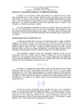
1 Anatomy of a Transmission Line Loudspeaker Martin J. King 40 Dorsman Dr. Clifton Park, NY 12065 Anatomy of a Transmission Line Loudspeaker By Martin J. King, 5/17/06 ( Revised 10/18/06) Copyright 2006 by Martin J. King. All Rights Reserved. Page 1 of 46 Introduction : For the past several years, I have been performing transmission line loudspeaker simulations using MathCad(1) computer models. When I started deriving the transmission line equations of motion I wanted to be able to easily simulate tapered, straight, and expanding geometries. To accommodate the geometry variable in the derivation, I merged the one dimensional exponential horn wave equation with a fiber damping correlation I had empirically formulated. The fiber damping model was generated using data acquired from measurements of the electrical impedance and the SPL output of a straight test transmission line.

2 The details of the transmission line modeling can be found on my website ( ). There have been two or three major revisions to my MathCad transmission line models in the past couple of years. Some of the changes corrected errors in the derived equations while others extended the capabilities of the worksheets to represent additional types of enclosures. Since September of 2000, versions of the MathCad worksheets have been available for downloading and have received wide use by transmission line and TQWT DIY speaker building enthusiasts. To the best of my knowledge, the speakers built based on these MathCad worksheets have been very successful and performance measurements correlate extremely well with the MathCad simulation predictions. While people have been applying my calculation methods to design transmission line loudspeakers for several years, there are always questions posted on Internet discussion forums or asked directly through private e-mails concerning how the transmission line enclosure actually functions.

3 For example, questions concerning the electrical impedance curve and if it is a double or a single humped curve are often posed. A second significant point of discussion revolves around the resonances of the air column and the Quarter wavelength frequencies and standing wave shapes. Over the years I have provided my responses to these two questions, and also to a host of other inquiries, by responding on discussion forums or by return e-mail. I decided recently that a useful document might be one that pulls some of these responses together and expands them to describe the inner workings of a transmission line enclosure. The result is this article which I have titled Anatomy of a Transmission Line Loudspeaker. I hope that the reader finds it both interesting and informative. Displacement, Velocity, and Acceleration : Three expressions need to be defined to allow the discussion to proceed and hopefully have some physical meaning for most readers.

4 In the following paragraphs sinusoidal displacement, velocity, and acceleration will be referred to over and over again. For example, the equations describing one possible sinusoidal displacement function and its relationship to velocity and acceleration are shown below. displacement = x(t) = sin( t ) velocity = u(t) = dx/dt = cos( t) = sin( t + 90 degrees) acceleration = a(t) = d2x/dt2 = - 2 sin( t) = 2 sin( t + 180 degrees) Anatomy of a Transmission Line Loudspeaker By Martin J. King, 5/17/06 ( Revised 10/18/06) Copyright 2006 by Martin J. King. All Rights Reserved. Page 2 of 46 In all of these expressions, the frequency has units of radians per second and is related to the more commonly used frequency variable f, having units of Hz or cycles per second, by the following expression. = 2 f Reviewing the expressions for displacement, velocity, and acceleration; it is observed that each time you differentiate with respect to time the magnitude increases by a factor of and the phase shifts by 90 degrees.

5 To help visualize a sinusoidal displacement, and the act of shifting it on the time axis by 90 degrees and 180 degrees to produce velocity and acceleration respectively, a sample plot is shown below in Figure 1. The magnitudes of the displacement and velocity curves have been scaled to produce a more easily visible comparison. Figure 1 : Displacement, Velocity, and Acceleration Curves Red curve = displacement = x(t) Blue curve = velocity = u(t) Magenta curve = acceleration = a(t) For the plot shown in Figure 1, the frequency was set equal to 1 Hz so that 90 degree and 180 degree phase shifts correspond to and seconds respectively on the time axis. Notice that the blue velocity curve is 90 degrees out of phase and that the magenta acceleration curve is 180 degrees out of phase with the red displacement curve. Recognizing the magnitude and phase relationships between the displacement, the velocity, and the acceleration is a key point to take away from this section.

6 Frequently consulting the curves shown in Figure 1 should help when trying to understand what is being described in subsequent sections. Anatomy of a Transmission Line Loudspeaker By Martin J. King, 5/17/06 ( Revised 10/18/06) Copyright 2006 by Martin J. King. All Rights Reserved. Page 3 of 46 Mechanical Vibration Theory : One Degree of Freedom System : To appreciate how a transmission line enclosure works, a little background information about mechanical vibration theory is required. The starting point for this section is the single degree of freedom system as shown in Figure 2. A single degree of freedom system is comprised of a mass, a damper, and a spring. Motion is allowed only in a single direction, in this case the vertical direction. The mass moves up and down at one end of the spring and damper while the other ends are anchored to ground. The mass has a displacement, velocity, and acceleration as described in the preceding section.

7 The positive sign convention is denoted on the right side of the figure by the arrow pointing upward. Figure 2 : Single Degree of Freedom Mechanical System The equation of motion for the single degree of freedom system is shown below. Notice that this equation sums acceleration, velocity, and displacement terms to react a forcing function on the right side of the equals sign. For a unit sinusoidal forcing function, F is equal to 1 Newton. m d2x/dt2 + c dx/dt + k x = F cos( t ) In simple mechanical models typically a degree of freedom (or motion opportunity) is assigned to each lumped mass in the system. For the system shown in Figure 2, there is one mass hence a single degree of freedom and a single natural frequency. As the number of masses increases, so do the number of degrees of freedom and therefore the number of natural or resonant frequencies. For a continuous system, such as a column of air vibrating in the axial direction, the number of masses is infinite as are the number of resonant frequencies.

8 An undergraduate level vibration textbook(2, 3) will contain the complete derivation and solution of the differential equation of motion for the single degree of freedom system, so it will not be repeated. Instead, a sample problem will be used to calculate and plot the response of the mass when it is subjected to a 1 Newton sinusoidal Anatomy of a Transmission Line Loudspeaker By Martin J. King, 5/17/06 ( Revised 10/18/06) Copyright 2006 by Martin J. King. All Rights Reserved. Page 4 of 46 excitation sweeping the frequency range from 10 Hz to 100 Hz. To set up and perform the numerical simulation, a few key variables must first be defined. Assume the mass is 25 gm and that the system s natural frequency is 40 Hz. The natural frequency of a single degree of freedom system is calculated using the well-known equation shown below. fn = 1/2 (k / m)1/2 Knowing the mass and frequency allows the spring rate to be calculated.

9 The calculated spring rate is 1579 Newton/m. Finally, the damping value is set to produce a Q of 50 at the 40 Hz resonance. This is a very lightly damped mechanical system that can be subjected to a 1 Newton sinusoidal excitation and numerically solved at discrete frequencies using MathCad. This is the process I used to perform all of the simulations presented in this section. Figures 3, 4, and 5 show the displacement, velocity, and acceleration responses for this single degree of freedom system subjected to a unit sinusoidal excitation. There are several classic properties of each response curve that will be described in the following paragraphs. But before diving into the details of each particular curve, it should be noted that this is a linear analysis. Basically, this means that if the excitation force were doubled the displacement, velocity, and acceleration response would also double.

10 If the excitation force were halved, the response would also be halved. The numerical response, extracted from the curves shown in Figure 3, 4, or 5, can be scaled to determine the response of the system to any magnitude of sinusoidal forcing function. One other feature common to all three response plots is the system behavior at resonance. A sharp peak at 40 Hz is seen in all three of the response plots. This is typical of a lightly damped mechanical system. At the resonant frequency, a small excitation level will produce a greatly amplified response when compared to other frequencies. What is sometimes neglected is the sudden phase shift that occurs as the forcing function sweeps through the resonant frequency. In each response plot, a 180 degree phase shift occurs as the frequency sweep traverses the resonant frequency of 40 Hz. One example of a resonance that everybody has heard at one time or another is the tone produced by rubbing a crystal wine glass typically used at a formal reception.