AutoCAD Civil 3D Tutorial: Importing Survey Points

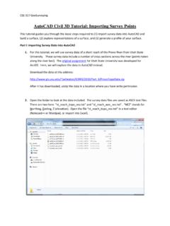
1 CEE 317 GeoSurveying AutoCAD Civil 3D Tutorial: Importing Survey Points This tutorial guides you through the basic steps required to (1) import Survey data into AutoCAD and build a surface, (2) explore representations of a surface, and (3) generate a profile of your surface. Part I: Importing Survey Data into AutoCAD 1. For this tutorial, we will use Survey data of a short reach of the Provo River from Utah State University. These Survey data include a number of cross sections across the river ( Points taken along the river bed). The original assignment for Utah State University was developed for ArcGIS. Here, we will explore the data in AutoCAD instead. Download the data at this address: ~jwheaton/ICRRR/2010/Part_ After it has downloaded, unzip the data in a location where you have write permission. 2. Open the folder to look at the data included.

2 The Survey data files are saved as ASCII text files. There are two here: and . NEZ stands for Northing, Easting, Z (elevation). Open the file in a text editor (Notepad++ or Wordpad, or import into Excel). CEE 317 GeoSurveying 3. You will find that this file has three columns, and these correspond to (1) the Northing, (2) the Easting, and (3) the elevation of each point (row). This file does not tell us the coordinate system of the Points or the units. In practice, you would consult with your surveying team to obtain the coordinate system and units of these data. In this example, this information is included in a metadata file ( ) which indicates these are in the Universal Transverse Mercator (UTM) projected coordinate system with units of meters. 4. Close any open text files. We are now ready to import into AutoCAD Civil 3D.

3 5. Launch AutoCAD Civil 3D English Metric (we know the units are in metric for this example) from the Start Menu (as seen below). Your machine may need to install the software let it do so. Note: It is important that you launch AutoCAD Civil 3D and not the original AutoCAD . Civil 3D has tools that are needed for this exercise that are not found in the original AutoCAD . CEE 317 GeoSurveying 6. AutoCAD Civil 3D will start. Close the welcome screen if it appears. 7. We will first create a Surface Definition. This is where the surveyed Points will be stored in the database. On the Home ribbon, click Surfaces > Create Surface. CEE 317 GeoSurveying 8. The Create Surface dialog appears. Here you can specify the name, description, default contour style, and render material for your surface. You will be able to change the Style and Render material later, so don t worry too much about them right now.

4 Make sure your screen matches the following graphic and click OK. 9. Now we have a surface database to store the Survey Points , but it is currently empty. Let s import the Survey Points now. Click the Modify Tab > Surface 10. The Surface tab now appears. Click Add Data > Point Files CEE 317 GeoSurveying 11. The Add Point File dialog appears. You should first note that there are many different format options in the Specify point file format window. Many of these are intuitive: P= point number, N = northing, E = easting, Z = elevation, D=description. You will also note that there are different ways to delimit the file, and these include: tab delimited, comma delimited, and space delimited. From Step 3 (above), you should have noted that the format is NEZ, and the columns are separated by a single space. Hit the plus sign next to the selected files window and browse to.

5 The tool should automatically detect NEZ (space delimited), but if it does not, select it in the file format window. Make sure your screen matches the options below and click OK. CEE 317 GeoSurveying 12. You may receive a warning that 1 point was outside the elevation extents this is probably the first row, which has a mysterious value of 5182 . Zoom extents if necessary to see your Points . AutoCAD is displaying the contours of your surface (1m minor interval, 5m major interval). You can see a meandering river! The green boundary represents the limits of your surface triangulation. In the next section you will explore ways of visually representing the surface. Part II: Representing the Surface 13. Now we will examine different ways to represent the surface. Click Modify > Surface to arrive at the Surface ribbon.

6 Then click Surface Properties > Surface Properties CEE 317 GeoSurveying 14. The Surface style dropdown provides several ways of visualizing your surface. We setup the surface to display Contours 1m and 5m . How else can we visualize the surface? First, let s examine the triangulations used to create the surface. Select Contours and Triangles and click Apply. The screen now shows how the surface was created and every triangulation calculation used between the Survey Points . The more dense the web, the more dense the number of Survey Points in an area. Inspecting this triangulated irregular network (TIN) is especially useful if the generated surface shows something unexpected, which may arise due to a surveying error or in areas that are not adequately surveyed. This is an important visualization tool, because it shows the location of your surveyed Points (at the vertices of the web).

7 You could surmise that there may be inaccuracies in the locations with less Survey Points . You can specify the shape of the boundary used to create this TIN surface. For example, you may want to move the boundary in closer to the river where you have more Survey Points . This is left for you as a future exercise. CEE 317 GeoSurveying 15. Now let s look at a raster-type representation of the surface. In the Surface Properties dialog, select Elevation Banding (2D) in the Surface style window and click Apply. AutoCAD should display a colorful representation of your surface, as seen below. We expect the red areas are the lowest elevations and the blue areas are the higher elevations, but how can we know for sure? Note that we can also view a similar map with the slope values ( Slope Banding 2D ). 16. To answer that question, let s return to the original representation select Contours 1m and 5m (Background) and hit Apply.

8 An easy (and intuitive) way to find the highest elevations and lowest elevations is to simply label the contours. Click Add Labels > Contours Multiple. Note that there are several options for labeling your surface here. CEE 317 GeoSurveying 17. Click a point in the top right area and move the mouse. You will see that a line follows your mouse. All contours that intersect this line will be labeled. Select a second point (as shown below) and hit enter. Zooming in, we find the following: As expected, the slope is draining to the river from both sides (1666 m to 1665 m). CEE 317 GeoSurveying 18. Now use the contour labeling tool to label the contours in the lower left extent. Zoom in after executing this tool, and we find the following: The contours in the lower left are around 1663 m. So this verifies that the river is flowing here from the top right to the bottom left.

9 (of course, you could have easily verified this with a field trip or a discussion with your Survey crew) A final note: the contour intervals here seem too large for this dataset. You can change the contour intervals in the Surface Properties dialogue (you will have to create a new style). CEE 317 GeoSurveying Part III: Creating a Profile from your Surface 19. Now that you have created a surface from your Survey Points and explored different ways of representing the surface visually, a useful exercise is to look at profiles (or cross sections) of your surface. This is especially important in design work where you are interested in how the topography varies along some path, which is called an alignment in AutoCAD . As an example, we will create a profile of the surface along the approximate route of the Provo River. To do this, we first need an alignment, which can be created from a polyline.

10 Zoom to the upper right part of the surface, and then type the command pl to start a new polyline. Click a point in the river to start the line, and then follow the meandering river, clicking along the way to add new vertices (as seen below). Do your best to follow the low Points of the river. In practice, you would probably want to pick a more refined way of tracing the river route, but we will just create the alignment manually here as an example. CEE 317 GeoSurveying 20. Once you have reached the end of the river, hit ENTER to finish the polyline. Left click on the polyline to select it. Note: if you made a mistake, you can either edit vertices with the polyline edit tool (type pe ) or you can delete the polyline and start over. 21. Make sure you are viewing the Home ribbon. With the polyline selected, hit Alignment > Create Alignment from Objects.