Transcription of B747 Cnb locus - Cornell University
1 Chapter 5 Dynamic StabilityThese notes provide a brief background for the response of linear systems, with applica-tion to the equations of motion for a flight vehicle. The description is meant to providethe basic background in linear algebra for understanding modern tools for analyzing theresponse of linear systems, and provide examples of their application to flight vehicledynamics. Examples for both longitudinal and lateral/directional motions are provided,and simple, lower-order approximations to the various modes are used to elucidate theroles of relevant aerodynamic properties of the Mathematical An Introductory ExampleThe most interesting aircraft motions consist of oscillatory modes, the basic features of which canbe understood by considering the simple system, sketched inFig.
2 , consisting of a spring, mass,and (t)kcxFigure : Schematic of spring-mass-damper 5. DYNAMIC STABILITYThe dynamics of this system are described by the second-order ordinary differential equationmd2xdt2+cdxdt+kx=F(t)( )wheremis the mass of the system,cis the damping parameter, andkis the spring constant ofthe restoring force. We generally are interested in both thefree responseof the system to an initialperturbation (withF(t) = 0), and theforced responseto time-varyingF(t). The free response isrelevant to the question of stability , the response toan infinitesimal perturbation from anequilibrium state of the system, while the forced response is relevant to control free response is the solution to the homogeneous equation, which can be writtend2xdt2+ cm dxdt+ km x= 0( )Solutions of this equation are generally of the formx=Ae t( )whereAis a constant determined by the initial perturbation.
3 Substitution of Eq. ( ) into thedifferential equation yields thecharacteristic equation 2+ cm + km = 0( )which has roots = c2m s c2m 2 km ( )The nature of the response depends on whether the second termin the above expression is real orimaginary, and therefore depends on the relative magnitudes of the damping parametercand thespring constantk. We can re-write the characteristic equation in terms of a variable defined by theratio of the two terms in the square root c2m 2 km =c24mk 2( )and a variable explicitly depending on the spring constantk, which we will choose (for reasons thatwill become obvious later) to bekm 2n( )In terms of these new variables, the original Eq.
4 ( ) can bewritten asd2xdt2+ 2 ndxdt+ 2nx= 0( )The corresponding characteristic equation takes the form 2+ 2 n + 2n= 0( )and its roots can now be written in the suggestive forms = n np 2 1 for >1 nfor = 1 n i np1 2for <1( ) MATHEMATICAL BACKGROUND77 Overdamped SystemFor cases in which >1, the characteristic equation has two (distinct) real roots, and the solutiontakes the formx=a1e 1t+a2e 2t( )where 1= n +p 2 1 2= n p 2 1 ( )The constantsa1anda2are determined from the initial conditionsx(0) =a1+a2 x(0) =a1 1+a2 2( )or, in matrix form, 1 1 1 2 a1a2 = x(0) x(0) ( )Since the determinant of the coefficient matrix in these equations is equal to 2 1, the coefficientmatrix is non-singular so long as the characteristic values 1and 2are distinct which is guaranteedby Eqs.
5 ( ) when >1. Thus, for theoverdampedsystem ( >1), the solution is completelydetermined by the initial values ofxand x, and consists of a linear combination of two reciprocal of theundamped natural frequency nforms a natural time scale for this problem,so if we introduce the dimensionless time t= nt( )then Eq. ( ) can be writtend2xd t2+ 2 dxd t+x= 0( )which is seen to depend only on the damping ratio . Figure shows the response of overdampedsystems for various values of the damping ratio as functionsof the dimensionless time Damped SystemWhen the damping ratio = 1, the system is said to becritically damped, and there is only a singlecharacteristic value 1= 2= n( )Thus, only one of the two initial conditions can, in general,be satisfied by a solution of the forme , in this special case it is easily verified thatte t=te ntis also a solution of Eq.
6 ( ), sothe general form of the solution for the critically damped case can be written asx= (a1+a2t)e nt( )The constantsa1anda2are again determined from the initial conditionsx(0) =a1 x(0) =a1 1+a2( )78 CHAPTER 5. DYNAMIC STABILITY02468101214161820 time, n tDisplacement, x = 1 = 2 = 5 = 1002468101214161820 time, n tDisplacement, x = 1 = 2 = 5 = 10(a)x(0) = (b) x(0) = : Overdamped response of spring-mass-damper system. (a) Displacement perturbation:x(0) = ; x(0) = 0. (b) Velocity perturbation: x(0) = ;x(0) = , in matrix form, 1 0 11 a1a2 = x(0) x(0) ( )Since the determinant of the coefficient matrix in these equations is always equal to unity, thecoefficient matrix is non-singular.
7 Thus, for thecritically dampedsystem ( = 1), the solution isagain completely determined by the initial values ofxand x, and consists of a linear combinationof a decaying exponential and a term proportional tote nt. For any positive value of ntheexponential decays more rapidly than any positive power oft, so the solution again decays, and include the limiting case of critically damped response for Eq. ( ).Underdamped SystemWhen the damping ratio <1, the system is said to beunderdamped, and the roots of the charac-teristic equation consist of the complex conjugate pair 1= n +ip1 2 2= n ip1 2 ( )Thus, the general form of the solution can be writtenx=e ntha1cos np1 2t +a2sin np1 2t i( )The constantsa1anda2are again determined from the initial conditionsx(0) =a1 x(0) = na1+ np1 2a2( )or, in matrix form, 10 n np1 2 a1a2 = x(0) x(0) ( )
8 MATHEMATICAL BACKGROUND7902468101214161820 1 time, n tDisplacement, x = = = = 102468101214161820 1 time, n tDisplacement, x = = = = 1(a)x(0) = (b) x(0) = : Underdamped response of spring-mass-damper system. (a) Displacement perturbation:x(0) = ; x(0) = 0. (b) Velocity perturbation: x(0) = ;x(0) = the determinant of the coefficient matrix in these equations is equal to np1 2, the systemis non-singular when <1, and the solution is completely determined by the initial values ofxand x. Figure shows the response of the underdamped system Eq.( ) for various values of thedamping ratio, again as a function of the dimensionless time is seen from Eq.
9 ( ), the solution consists of an exponentially decaying sinusoidal motion is characterized by its period and the rate at which the oscillations are damped. Theperiod is given byT=2 np1 2( )and the time to damp to 1/ntimes the initial amplitude is given by1t1/n=lnn n ( )For these oscillatory motions, the damping frequently is characterized by thenumber of cyclestodamp to 1/ntimes the initial amplitude, which is given byN1/n=t1/nT=lnn2 p1 2 ( )Note that this latter quantity is independent of the undamped natural frequency; , it dependsonlyon the damping ratio . Systems of First-order EquationsAlthough the equation describing the spring-mass-damper system of the previous section was solvedin its original form, as a single second-order ordinary differential equation, it is useful for later1 The most commonly used values ofnare 2 and 10, corresponding to the times to damp to 1/2 the initial amplitudeand 1/10 the initial amplitude, 5.
10 DYNAMIC STABILITY generalization to re-write it as asystemof coupled first-order differential equations by definingx1=xx2=dxdt( )Equation ( ) can then be written asddt x1x2 = 01 2n 2 n x1x2 + 01m F(t)( )which has the general form x=Ax+B ( )wherex= (x1,x2)T, the dot represents a time derivative, and (t) =F(t) will be identified as thecontrol free response is then governed by the system of equations x=Ax( )and substitution of the general formx=xie it( )into Eqs. ( ) requires(A iI)xi= 0( )Thus, the free response of the system in seen to be completelydetermined by the eigenstructure ( ,the eigenvalues and eigenvectors) of theplant matrixA.