Brownian Motion and An Introduction to Stochastic Integration

1 Brownian Motion andAn Introduction to Stochastic IntegrationArturo FernandezUniversity of California, BerkeleyStatistics 157: Topics In Stochastic Processes SeminarMarch 10, 20111 IntroductionIn the world of Stochastic modeling, it is common to discuss processes with dis-crete time intervals. Brownian Motion (BM) is the realization of a continuous timestochastic process. Furthermore, the continuity of BM is an important propertythat develops a basis for Stochastic intgeration. What is Stochastic intgeration?In introductory calculus, the concept of Integration is usually done with respectto variables that are fixed. Real Analysis explores the topic of Integration withrespect to functions of the same parameter.

2 Most variations of Stochastic inte-gration integrate Stochastic processes with respect to an independent brownianmotion. However, most Stochastic differential equations (SDEs) have no specificway from which we can can find a closed-form solution and we must apply nu-merical techniques to generalize the shape of solution. In this paper, I introduceand construct Brownian Motion via a random walk process and then note someof its properties. Finally, I give a rough preview into Stochastic Integration withtheory and examples of numerical methods for solving The Random Walk Revisited: ConstructingBrownian Motion (Note: The following Introduction to the Wiener process, its properties, and the extended generalizationis based off the lecture notes referred to in [1].)

3 Let{ k}k Nbe a sequence of independent and identically distributed ( ) dis-crete random variables such thatP{ k= 1}= 1/2. Note thatE[ k] = 0 and Var[ k] =E[ 2k]= 1and defineS0= 0 andSn=n k=1 k1 Fernandez2As a funtion of discrete timen,Snis the position of a random walk (p=12,q=12)onZ. Suppose we want to rescale time and space so that we have a stochasticprocess ont [0,1] and with values inR. We can construct such a thing via anapplication of the Central Limit Theorem:That is, asN ,SN Nconverges in distribution to a standard normaldistribution,SN N k k N=SN Nd N(0,1)(1)Thus, we can define a piecewise constant, random functionWNtont [0,1] bylettingWNt=SbN tc N(2)whereb cis the integer-floor function.

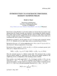
4 As per standard notation for stochasticprocesses, we have written the time parametertof the random function as a sub-script, (t). 1: Realizations ofWNtforN= 75 (red),N= 300 (green),andN= 5000 (blue)Theorem 1(Donsker).AsN ,WNtconverges in distribution to a stochasticprocessWtWNtd Wt(3)Wtis termed as the Wiener Process or also Brownian ,Wt=W(t), is a random function with time parametert. Theorem 1will go without proof in this discussion. We will continue by taking for grantedthat the limiting processWtexists and study its Properties Basic PropertiesThe Wiener processWthas the following basic properties:(a)Independence:Wt Wsis independent of{W } s 0 s t(b)Stationarity(Stationary Increments):The statistical distribution ofWt+s Wsis independedent ofs(andtherefore equivalent in distribution toWt.)

5 (c)Gaussianity:Wtis a Gaussian Process with:MeanE(Wt) = 0andCovarianceE(Wt Ws) = min(t,s)(d)Continuity:With probabaility 1,Wtviewed as a function oftis continuous. ( set of discontinuities has measure zero) Sketch Proof of Basic Independence and StationarityTo show independence (a) and stationarity (b), first note that for 1 m n,Sn Sm=n k=m+1 kis independent ofSmand equal in distribution toSn msince the k s are , it follows that for 0 s t,Wt Wsis independent ofWsand thatWt Wsd=Wt s(4) GaussianityTo show Gaussianity (c), we check thatWtis in fact a Gaussian Process byfinding its probability density function (pdf) at a timetand then establishing 0.

6 AsN ,WNt=SbNtc N=SbNtc bNtc bNtc Nd N(0,1) td=N(0,t)(5)Fernandez4 This gives us an idea of the distribution of values ofWtas it evolves over , we can interpret (5), for a fixed timet, asP(Wt [x1,x2]) = x2x1 (x,t)dx(6)= x2x1e x2/2t 2 tdx(7)Note that (x,t) is simply defined by the scaling of a Gaussian distribution, where = 0 and = t. As such, (x,t) =1 2 e (x )22 2=e x2/2t 2 tis the probability density function (pdf) forWtat a fixed understand the Gaussian properties ofWt, we begin with the following. LetP={0< t1 t2 .. tn}be a partition of (0,1]. Then, the vector (WNt1,..,WNtn) will converge in distribu-tion to an-dimensional Gaussian variable.)

7 Furthermore, the probability densitythat (Wt1,..,Wtn) = (x1,..,xn) can be derived, using the independence andstationarity of incerements ofWt:Pd(Wt1=x1,..,Wtn=xn) =Pd(Wt1=x1,Wt2 Wt1=x2 x1,..,Wtn Wtn 1=xn xn 1)=Pd(Wt1=x1,Wt2 t1=x2 x1,..,Wtn tn 1=xn xn 1)Therefore, (x1,t1) (x2 x1,t2 t1) (xn xn 1,tn tn 1) is the probabilitydensity referred to addition, we derive the expectation and covariance of the Gaussian :E[Wt] = 0E[Wt] = Rx (x,t) = Rodd even= 0 Covariance:Cov(Wt,Ws) = min(t,s) prove the case when 0 s tand show that Cov(Wt,Ws) =s. Thecase when 0 t sfollows in a similar manner and proves the desired 0 s t. SinceW0= 0 and the increments ofWtare independent,Cov(Wt,Ws) =E[Wt Ws]=E[(Ws+Wt Ws)Ws]=E[(W2s+ (Wt Ws)Ws]=E[W2s] +E[(Wt Ws)Ws]=s+E[(Wt Ws)(Ws W0)]=s+E[Wt Ws] E[Ws W0]=s+E[Wt Ws] E[Ws]=s+E[Wt Ws](0)= Other Self-similarityThe Wiener Process is self-similar, in the sense that for >0,Wtd= 1/2W t(8)Therefore, studying it on [0,1] will provide us with enough information to deduceits properties on any interval.)

8 The proof of (8) follows by showing that 1/2W tis a Gaussian Process with the same mean and covariance as the Wiener that a processG(t) is a Gaussian processs if and only if any finite linearcombination of samples of the Gaussian process will be normally isG(t) is a iaiG(ti) is Gaussian(9)forai,tiusually inR. Therefore, if we define some new processH(t) =a(t)G(c(t))note that iaiH(ti) = iai a(ti)G(c(ti))= i aiG( ti)It follows that 1/2W tis in fact a Gaussian process. Its mean and covarianceare easily calculated using the same techniques we used for the Wiener First Passage TimesGivena >0, we define the first passage time forato beTa:= inf{t:Wt=a}.

9 Claim (Wt> a) =12P(Ta< t)(10) the following second equality follows by the continuity ofWtandthe third by symmetry ofWt,P(Wt> a) =P(Wt> a)=P(Ta< t,Wt> a)=12P(Ta< t)DefineMt= sup0 s tWsandmt= inf0 s tWs. Note that by (10)P(Mt> a) =P(Ta< t) = 2P(Wt> a) = 2 ae x2/2t 2 tdx(11)Similarly, by a symmetric argument it follows thatP(Mt> a) =P(mt< a). Wenow shortly divert from the topic of Brownian Motion to introduce some conceptsin Stochastic Foundation for Stochastic Integrals(Note: The following Introduction to Stochastic integrals is based off the lecture notes referred to in [2].) Motivation from Real AnalysisSuppose we want to evaluateI(x) bax(t)dt.

10 From Real Analysis, we knowthat for a partitionP={a=t0< t1< < tn=b}ofnintervals and awell-behaved functionx(t) that its Riemann Intergral, defined by a left endpointapproximation,In(x) n i=1x(ti 1)(ti ti 1)(12)will converge toI(x) asn and mesh(P) 0, where mesh(P)= max{ti ti 1:1 i n}. Now suppose we would like to evaluate the integral ofx(t) with respectto some functionw(t)Iw(x) = bax(t)dw(t)(13)Ifwis differentiable on [a,b], then by change of variablesIw(x) = bax(t)w (t) this case, the approximating sum is now of the formn i=1x(ti 1)w (ti 1)(ti ti 1)(14)Alternatively, for nicew(t), there is the Riemann-Stieltjes integral approximatingsumn i=1x(ti 1)(w(ti) w(ti 1))(15)Fernandez7which we can use even ifw doesn t with an example inR, suppose we want to approximate the solu-tion ofdx/dt=f(x).