Transcription of Chapter 1 Simple Linear Regression (part 4)
1 Chapter 1 Simple Linear Regression (part 4)1 Analysis of Variance (ANOVA) approach to regressionanalysisRecall the model againYi= 0+ 1Xi+ i,i=1, .., nThe observations can be written deviation of eachYifrom the mean Y,Yi YThe fitted Yi=b0+b1Xi,i=1, .., nare from the Regression and determined mean is Y=1nn i=1Yi= YThus the deviation of Yifrom its mean is Yi YThe residualsei=Yi Yi,withmeanis e=0(why?)Thus the deviation ofeifrom its mean isei=Yi Yi1 WriteYi Y Total deviation= Yi Y Deviationdue the Regression +ei Deviationdue to the errorobsdeviation ofdeviation ofdeviation ofYi Yi=b0+b1 Xiei=Yi Yi1Y1 Y Y1 Ye1 e=e12Y2 Y Y2 Ye2 e= Y Yn Yen e=enSum of ni=1(Yi Y)2 ni=1( Yi Y)2 ni=1e2isquaresTotal SumSum ofSum ofof squaressquares due tosquares ofregressionerror/residuals(SST)(SSR)(SS E)We haven i=1(Yi Y)2 SST=n i=1( Yi Y)2 SSR+n i=1e2i SSEP roof.
2 N i=1(Yi Y)2=n i=1( Yi Y+Yi Yi)2=n i=1{( Yi Y)2+(Yi Yi)2+2( Yi Y)(Yi Yi)}=SSR+SSE+2n i=1( Yi Y)(Yi Yi)=SSR+SSE+2n i=1( Yi Y)ei=SSR+SSE+2n i=1(b0+b1Xi Y)ei=SSR+SSE+2b0n i=1ei+2b1n i=1 Xiei 2 Yn i=1ei=SSR+SSEIt is also easy to checkSSR=n i=1(b0+b1Xi b0 b1 X)2=b21n i=1(Xi X)2(1)2 Breakdown of the degree of freedomThe degrees of freedom for SST isn 1: noticing thatY1 Y , .., Yn Yhave one constraint ni=1(Yi Y)=0 The degrees of freedom for SSR is 1: noticing that Yi=b0+b1Xi(see Figure 1) 101 Xresiduals eFigure 1: A figure shows the degree of freedomThe degrees of freedom for SSE isn 2: noticing thate1, .., enhave TWO constraints ni=1ei=0and ni=1 Xiei= 0 ( , the normal equation).Mean (of) SquaresMSR=SSR/1calledregression mean squareMSE=SSE/(n 2)callederror mean squareAnalysis of variance (ANOVA) tableBased on the break-down, we write it as a tableSource ofvariationSSdf MSF-valueP(>F) Regression SSR = ni=1( Yi Y)21 MSR=SSR1F =MSRMSEp-valueErrorSSE = ni=1(Yi Yi)2n-2 MSE =SSEn 2 TotalSST = ni=1( Yi Y)2n-13R command for the calculationanova(object.)
3 Where object is the output of a Mean SquaresE(MSE)= 2andE(MSR)= 2+ 21n i=1(Xi X)2[Proof: the first equation was proved (where?). By (1), we haveE(MSR)=E(b1)2n i=1(Xi X)2=[Var(b1)+(Eb1)2]n i=1(Xi X)2=[ 2 ni=1(Xi X)2+ 21]n i=1(Xi X)2= 2+ 21n i=1(Xi X)2]2F-testofH0: 1=0 Consider the hypothesis testH0: 1=0,Ha: 1 = that Yi=b0+b1 XiandSSR=b21n i=1(Xi X)2 Ifb1=0thenSSR= 0 (why). Thus we can test 1=0basedonSSR. underH0, SSRor MSR should be small .We consider the F-statisticF=MSRMSE=SSR/1 SSE/(n 2).UnderH0,F F(1,n 2)For a given significant level , our criterion is4 IfF F(1 ,1,n 2) ( indeed small), acceptH0 IfF >F(1 ,1,n 2)( not small), rejectH0whereF(1 ,1,n 2) is the (1 ) quantile of the F can also do the test based on the p-value =P(F>F ),If p-value , acceptH0If p-value< , rejectH0 Example the example above (withn= 25, in part 3), we fit a modelYi= 0+ 1Xi+ i(By(R code)), we have the following outputAnalysis of Variance TableResponse: YDf Sum Sq Mean Sq F valuePr(>F)X 1 252378 252378 **Residuals 23 54825 2384 Suppose we need to testH0: 1= 0 with significant level , based on the calculation,the p-value is 10 10< , we should ofF-test and t-testWe have two methods to testH0: 1=0versusH1: 1 = 0.
4 RecallSSR=b21 ni=1(Xi X) =SSR/1 SSE/(n 2)=b21 ni=1(Xi X)2 MSEBut sinces2(b1)=MSE/ ni=1(Xi X)2(where?), we have underH0,F =b21s2(b1)=(b1s(b1))2=(t ) >F(1 ,1,n 2) (t )2>(t(1 /2,n 2))2 |t |>t(1 /2,n 2).andF F(1 ,1,n 2) (t )2 (t(1 /2,n 2))2 |t | t(1 /2,n 2).(you can check in the statistical tableF(1 ,1,n 2) = (t(1 /2,n 2))2) Therefore,the test results based on F and t statistics are the same. (But ONLY for Simple linearregression model)53 General Linear test approachTo test whetherH0: 1= 0, we can do it by comparing two modelsFull mo del :Yi= 0+ 1Xi+ iandReduced model :Yi= 0+ iDenote the SSR of the FULL and REDUCED models bySSR(F)andSSR(R) respec-tively (and SSE(R), SSR(F)). We have immediatelySSR(F) SSR(R)orSSE(F) SSE(R).A question: when does the equality hold?
5 Note that ifH0: 1=0holds,thenSSE(R) SSE(F)SSE(F)should be smallConsidering the degree of freedoms, defineF=(SSE(R) SSE(F))/(dfR dfF)SSE(F)/dfFshould be smallwheredfRanddfFindicate the degrees of freedom ofSSE(R)andSSE(F) : 1=0,itisprovedthatF F(dfR dfF,dfF)Suppose we get theFvalue asF ,thenIfF F(1 , dfR dfF,dfF),acceptH0 IfF >F(1 , dfR dfF,dfF),rejectH0 Similarly, based on the p-value =P(F>F ),If p-value , acceptH0If p-value< , rejectH064 Descriptive measures of Linear association betweenXandYIt follows fromSST=SSR+SSEthat1=SSRSST+SSESST where SSRSSTis the proportion of Total sum of squares that can be explained/predicted by thepredictorX SSESSTis the proportion of Total sum of squares that caused by the random good model should have largeR2=SSRSST=1 SSESSTR2is calledR square,orcoefficient of determinationSome facts aboutR2for Simple Linear Regression model1.
6 0 R2 ifR2=0,thenb1= 0 (becauseSSR=b21 ni=1(Xi X)2)3. ifR2=1,thenYi=b0+b1Xi(why?)4. the correlation coefficient betweenrX,Y= R2[Proof:R2=SSRSST=b21 ni=1(Xi X)2 ni=1(Yi Y)2= indicates the fitness in the observed range/scope. We need to be careful if wemake prediction outside the indicates the Linear relationships .R2= 0 does not meanXandYhave nononlinear Considerations in Applying Regression analysis1. In prediction a new case, we need to ensure the model is applicable to the new Sometimes we need to predictX, and thus predictY. As a consequence, the predictionaccuracy also depends on the prediction ofX3. The range ofXfor the model. If a new caseXis far from the range, in the prediction,we need be careful4. 1 = 0 only indicates the correlation relationship, but not a cause-and-effect relation(causality).]
7 5. Even if 1= 0 can be concluded, we cannot sayYhas no relationship/associationwithX. We can only say there is no Linear relationship/association Write an estimated model Y=b0+b1X( )(s(b0))(s(b1)) 2(or MSE) = ..,R2= ..,F-statistic = .. (and others)Other formats of writing a fitted model can be found in Part 3 of the lecture