Transcription of Chapter 13 Distributed Feedback (DFB) Structures and …
1 Semiconductor Optoelectronics (Farhan Rana, Cornell University) Chapter 13 Distributed Feedback (DFB) Structures and Semiconductor DFB Lasers Distributed Feedback (DFB) Gratings in Waveguides Introduction: Periodic Structures , like the DBR mirrors in VCSELs, can be also realized in a waveguide, as shown below in the case of a InGaAsP/InP waveguide. In the waveguide shown above, periodic grooves have been etched in the top surface of the InGaAsP waveguide before the growth of the top InP layer. Such periodic grating Structures are examples of one dimensional photonic bandgap materials. The relative dielectric constant is a function of the z-coordinate and can be written as, ),,(),(),,(avgzyxyxzyx The average dielectric constant ),(avgyx corresponds to the waveguide structure shown below in which the grating region has been replaced by a layer with a z-averaged dielectric constant.
2 InP InP z=0 z=LInGaAsP waveguide InGaAsP/InP grating region a InP InP z=0 z=LInGaAsP InGaAsP/InP grating region replaced by a layer with a z-averaged dielectric constant Semiconductor Optoelectronics (Farhan Rana, Cornell University) The z-average of the part ),,(zyx is therefore zero. If the period of the grating is a, then one may expend ),,(zyx in terms of a Fourier series, 0,),,(pipGzpedyxfzyx where the reciprocal lattice vector (also called the grating vector) G equals a 2. If ),,(zyx is real then, *ppdd . yxf, equals one in the grating region and equals zero everywhere else. In the above Fourier series for ),,(zyx , usually the fundamental harmonic dominates and therefore we will assume that, iGziGzededyxfzyx 11,),,( A wave travelling in the waveguide with a wavevector can Bragg scatter from the periodic grating provided the conditions for Bragg scattering are satisfied, finalfinal G The only way these conditions can be satisfied in one dimension is when final, the wave is reflected in the opposite direction, effnaGG22 So a forward traveling wave will be Bragg reflected if its wavevetor is close to aG 2.
3 If we call this special wavevector o then aGo 2. We can write ),,(zyx as, ziziooededyxfzyx 2121,),,( Wave propagation in a DFB Grating Waveguide Coupled Mode Technique: One can analyze wave propagation in a DFB grating waveguide in two steps discussed below. Step 1: First consider the waveguide corresponding to ),(avgyx shown in the Figure above and solve for the eigemodes and the propagation vectors (eigenvalues) for all frequencies of interest. The eignemodes, zieyxE , and zieyxH , satisfy Maxwell s equations, zioziziozieyxEyxieyxHeyxHieyxE ,,,,,avg or, yxEyxiyxHziyxHiyxEziotot,,, ,, avg The above equations can be solved to give the mode effective index effn. Given a grating structure , we can now find the frequency o that will Bragg scatter from the relation, ancooeffoo If the wavevector is very different from o then the grating structure will likely not affect the solution much (there will be not much scattering).
4 The interesting case is when o . This case is discussed below. Semiconductor Optoelectronics (Farhan Rana, Cornell University) Step 2: We treat the part ),,(zyx as a perturbation. The perturbation will have the strongest affect when o . For o , we write the solution as, zizizizieyxHzAeyxHzAzyxHeyxEzAeyxEzAzyxE ,,,,,,,,** Here, the functions zA and zA are assumed to be slowly varying in space. The form of the solution allows for coupling between the forward and backward going waves because of Bragg scattering from the grating. The technique described below is called coupled mode theory. Plugging the assumed form of the solution in Maxwell s equations gives, zizizizioziziziziozizieyxEzAeyxEzAededyx fyxieyxHzAeyxHzAeyxHzAeyxHzAieyxEzAeyxEz Aoo ,, ,,,,,,,,*2121avg** Using the Maxwell s equation satisfied by the eigenmode we get, ziziziziozizizizieyxEzAeyxEzAededyxfiedz zdAyxHzedzzdAyxHzedzzdAyxEzedzzdAyxEzoo ,, ,, , 0, , *2121** We multiply the first equation above by yxH,* and multiply the second equation above by yxE,* and then subtract the two equations, and keep only the terms that are approximately phase matched to get on left and right hand sides to get.
5 ZAdxdyzyxHyxEyxHyxEdxdyyxEyxEyxfedidzzdA zioo .,,,,,.,,**21 If instead of subtracting, we add the two equations then we obtain, zAdxdyzyxHyxEyxHyxEdxdyyxEyxEyxfedidzzdA zioo .,,,,,.,,**21 If (and only if) ),,(zyx is real and *11dd , then the above two equations can be written as, zAzAeieizAzAdzdzizioo0*022 where the coupling constant is, G1**region Grating**12 .,,Re,.,,.,,.,2 gMgMgMgMgMgovnnddxdyzyxHyxEdxdyyxEyxEnnd xdyyxEyxEnndxdyyxEyxEnnnnd Here, Mgnn is the product of the index and the (material) group index of the grating region, gv is the group velocity of the mode, and the overlap integral G is the usual mode confinement factor for the grating region provided the mode electric field is real (for example, the mode electric field will be real Semiconductor Optoelectronics (Farhan Rana, Cornell University) if ),(avgyx is real and the z-component of the field is negligible).
6 The coupling constant couples the forward and the backward propagating waves. To solve the above set of equations, we assume, ziziooezAzBezAzB)()()()()()( )(zB and )(zB satisfy, )()(* )()()(*)()()(zBzBiiiizBzBiiiizBzBdzdoo We have a 2x2 linear system of equations. The eigenvalues of the matrix on the right hand sided are s where, iqs 22 iqs 22 The corresponding eigenvectors are, ississ The most general form of the solution is, siqsiqeisCeisCzBzBiqziqz 21)()( The constants 1C are 2C are determined by the boundary conditions. Note that in terms of )(zB and )(zB the electric field can be written as, ziziooezByxEezByxEzyxE )(),()(),(),,(* From the expression above, the effective propagation vector of, say the forward going wave, at frequency is not anymore but is k where, 2222 ooooqk The difference between the modal dispersions and k is depicted in the Figure below.
7 Note that a frequency gap (or a bandgap) opens in the dispersion relation of magnitude given by, ggv2 For values of frequency that fall in this bandgap, no real value of the propagation vector k satisfies the dispersion relation given above. ( ) ( ) Bandgap g (k) (k) Semiconductor Optoelectronics (Farhan Rana, Cornell University) DFB Waveguide Mirror (or a Distributed Bragg Reflector (DBR)): Consider a DFB structure as shown in the Figure below. We need to calculate the reflectivity of the mirror for a wave coming in inside the waveguide from the left side. The reflection and transmission coefficients are, 00 BBr LioeBLBt )0()( The boundary conditions are, 0 LB and 00 B. We need to find the constants 1C are 2C in, siqsiqeisCeisCzBzBiqziqz 21)()( in order to satisfy the above boundary conditions.
8 The final result is, )0()cosh()sinh()](sinh[*)()0()cosh()sinh ()](cosh[)](sinh[)( BsLissLLzszBBsLissLLzsisLzszB The reflection coefficient is, )cosh()sinh()sinh(*)0()0(sLissLsLBBr The transmission coefficient is, LiLiooesLissLiseBLBt )cosh()sinh()0()( The magnitude of the reflection coefficient is maximum when the wavevector of the incident wave is equal to o and 0 , LRLir 2max0tanhtanh* The Figure below plots the reflectivity of a DBR mirror as a function of the wavelength (or wavevector) for different values of the coupling constant. Note that the reflection coefficient r goes to zero when, 222222222)()(integer nonzero LnLnninsLo z=0 z=LB+(0) B-(0) B+(L)B-(L)Semiconductor Optoelectronics (Farhan Rana, Cornell University) The first zero in the reflection on either side of o determines the bandwidth over which the DBR mirror is an effective reflector.
9 This bandwidth DBR is, 22 DBR22 DBR22 LvLg An infinitely long DFB structure is a one dimensional photonic bandgap material. The stopband or the bandgap g of this material is, gLgv2 DBR In crystals, the bandgap in the electron energy spectrum comes about as a result of the Bragg scattering of electrons from the periodic atomic potential and the magnitude of the bandgap is proportional to the strength of the scattering potential. In DFB Structures , the photonic bandgap also results from the Bragg scattering of electromagnetic waves from the periodic index of the medium, and the strength of the bandgap also depends on the strength of the index variations as captured by the coupling constant . Distributed Feedback (DFB) Lasers (1D Photonic Crystal Lasers) Introduction: The structure of a DFB laser is shown in the Figures below.
10 The laser cavity is not like any we have seen before. There is no distinction between the optical cavity and the mirrors. The DFB grating provides back reflection that keeps the photons from escaping from the two end facets. The facets are assumed to be perfectly AR coated and provide no reflection. The laser cavity minors are Distributed along the entire length of the cavity. The techniques developed in the last section are adequate to analyze lasing in DFB lasers. Analyzing a laser involves at least: (i) finding the frequencies of the lasing modes, (ii) finding the threshold gain thg~ and the photon lifetime of each mode, and (iii) finding the output coupling efficiency o . Semiconductor Optoelectronics (Farhan Rana, Cornell University) DFB Laser Analysis: For the waveguide cavity shown above, photon lifetime is related to the threshold gain thg~ by the familiar relation: pthgagv 1~ Photon lifetime is related to the two different kinds of losses; mirror or external losses, and cavity internal losses, )~~(1 mgpv To analyze the DFB laser shown above, we first assume 0~ ( no material losses in any region) and calculate the threshold gain, thg~.