Transcription of CHAPTER 3 ANTENNA ARRAYS AND BEAMFORMING
1 CHAPTER 3. ANTENNA ARRAYS AND BEAMFORMING . Array beam forming techniques exist that can yield multiple, simultaneously available beams. The beams can be made to have high gain and low sidelobes, or controlled beamwidth. Adaptive beam forming techniques dynamically adjust the array pattern to optimize some characteristic of the received signal. In beam scanning, a single main beam of an array is steered and the direction can be varied either continuously or in small discrete steps. ANTENNA ARRAYS using adaptive BEAMFORMING techniques can reject interfering signals having a direction of arrival different from that of a desired signal. Multi- polarized ARRAYS can also reject interfering signals having different polarization states from the desired signal, even if the signals have the same direction of arrival.
2 These capabilities can be exploited to improve the capacity of wireless communication systems. This CHAPTER presents essential concepts in ANTENNA ARRAYS and BEAMFORMING . An array consists of two or more ANTENNA elements that are spatially arranged and electrically interconnected to produce a directional radiation pattern. The interconnection between elements, called the feed network, can provide fixed phase to each element or can form a phased array. In optimum and adaptive BEAMFORMING , the phases (and usually the amplitudes) of the feed network are adjusted to optimize the received signal. The geometry of an array and the patterns , orientations, and polarizations of the elements influence the performance of the array. These aspects of array antennas are addressed as follows.
3 The pattern of an array with general geometry and elements is derived in Section ; phase- and time-scanned ARRAYS are discussed in Section Section gives some examples of fixed BEAMFORMING techniques. The concept of optimum BEAMFORMING is introduced in Section Section describes adaptive algorithms that iteratively approximate the optimum BEAMFORMING solution. Section describes the effect of array geometry and element patterns on optimum BEAMFORMING performance. Pattern of a Generalized Array A three dimensional array with an arbitrary geometry is shown in Fig. 3-1. In spherical coordinates, the vector from the origin to the nth element of the array is given L. by rm = ( m , m , m ) and k = (1, , ) is the vector in the direction of the source of an 29.
4 Incident wave. Throughout this discussion it is assumed that the source of the wave is in the far field of the array and the incident wave can be treated as a plane wave. To find the array factor, it is necessary to find the relative phase of the received plane wave at each element. The phase is referred to the phase of the plane wave at the origin. Thus, 2 . the phase of the received plane wave at the nth element is the phase constant =.. L. multiplied by the projection of the element position rm on to the plane wave arrival L L. vector k . This is given by k rm with the dot product taken in rectangular coordinates. z incident wave mth element -k rm y . x Figure 3-1. An arbitrary three dimensional array In rectangular coordinates, k = sin cos x + sin sin y + cos z = r and L.
5 Rm = m sin m cos m x + m sin m sin m y + m cos m z , and the relative phase of the incident wave at the nth element is L L. m = k rm = m (sin cos sin m cos m + sin sin sin m sin m + cos cos m ) ( ). = ( x m sin cos + y m sin sin + z m cos ). Array factor For an array of M elements, the array factor is given by 30. M. AF ( , ) = I m e j ( m + m ) ( ). m =1. where I m is the magnitude and m is the phase of the weighting of the mth element. The normalized array factor is given by AF ( , ). f ( , ) = ( ). max{ AF ( , ) }. This would be the same as the array pattern if the array consisted of ideal isotropic elements. Array pattern If each element has a pattern g m ( , ) , which may be different for each element, the normalized array pattern is given by M.
6 I m g m ( , )e j ( m + m ). F ( , ) = m =1. ( ). M . max I m g m ( , )e j ( m + m ) . m =1 . In ( ), the element patterns must be represented such that the pattern maxima are equal to the element gains relative to a common reference. Phase and Time Scanning Beam forming and beam scanning are generally accomplished by phasing the feed to each element of an array so that signals received or transmitted from all elements will be in phase in a particular direction. This is the direction of the beam maximum. Beam forming and beam scanning techniques are typically used with linear, circular, or planar ARRAYS but some approaches are applicable to any array geometry. We will consider techniques for forming fixed beams and for scanning directional beams as well as adaptive techniques that can be used to reject interfering signals.
7 Array beams can be formed or scanned using either phase shift or time delay systems. Each has distinct advantages and disadvantages. While both approaches can be used for other geometries, the following discussion refers to equally spaced linear ARRAYS 31. such as those shown in Fig. 3-2. In the case of phase scanning the interelement phase shift is varied to scan the beam. For time scanning the interelement delay t is varied. 1 2 M. 1 2 M.. A1 A2 AM. A1 A2e j . AMe j(M-1) . t (M-1) t . to receiver to receiver (a) (b). Figure 3-2. (a) a phase scanned linear array (b) a time-scanned linear array Phase scanning Beam forming by phase shifting can be accomplished using ferrite phase shifters at RF or IF. Phase shifting can also be done in digital signal processing at baseband.
8 For an M-element equally spaced linear array that uses variable amplitude element excitations and phase scanning the array factor is given by [ ]. M 1 2 d jm ( cos + ). AF ( ) = Am e . ( ). m=0. where the array lies on the x-axis with the first element at the origin. The interelement phase shift is 2 d = cos 0 ( ). 0. 32. and 0 is the wavelength at the design frequency and 0 is the desired beam direction. At a wavelength of 0 the phase shift corresponds to a time delay that will steer the beam to 0. In narrow band operation, phase scanning is equivalent to time scanning, but phase scanned ARRAYS are not suitable for broad band operation. The electrical spacing (d/ ) between array elements increases with frequency. At different frequencies, the same interelement phase shift corresponds to different time delays and therefore different angles of wave propagation, so using the same phase shifts across the band causes the beam direction to vary with frequency.
9 This effect is shown in Fig 3-3. This beam squinting becomes a problem as frequency is increased, even before grating lobes start to form. 8. 7 f0. 2f0. 6. 5. |AF(phi)|. 4. 3. 2. 1. 0. 0 50 100 150 200. phi, degrees Figure 3-3. Array factor of 8-element phase-scanned linear array computed for three frequencies (f0, , and 2f0), with d= at f0, designed to steer the beam to o=45 at f0. 33. Time scanning Systems using time delays are preferred for broadband operation because the direction of the main beam does not change with frequency. The array factor of a time- scanned equally spaced linear array is given by M 1 2 d jm ( cos + t ). AF ( ) = Am e . ( ). m =0. where the interelement time delay is given by d t = cos 0 ( ). c Time delays are introduced by switching in transmission lines of varying lengths.
10 The transmission lines occupy more space than phase shifters. As with phase shifting, time delays can be introduced at RF or IF and are varied in discrete increments. Time scanning works well over a broad bandwidth, but the bandwidth of a time scanning array is limited by the bandwidth and spacing of the elements. As the frequency of operation is increased, the electrical spacing between the elements increases. The beams will be somewhat narrower at higher frequencies, and as the frequency is increased further, grating lobes appear. These effects are shown in Fig. 3-4. 34. 8. f0. 7 2f0. 6. |AF(phi)| 5. 4. 3. 2. 1. 0. 0 50 100 150 200. phi, degrees Figure 3-4 Array factor of 8-element time-scanned linear array computed for three frequencies (f0, , and 2f0), with d= at f0, designed to steer the beam to o=45 at f0.