Chapter 3 Classical Variational Methods and the Finite ...

1 44 Chapter 3: Classical Variational Methods and the Finite Element Method Introduction Deriving the governing dynamics of physical processes is a complicated task in itself; finding exact solutions to the governing partial differential equations is usually even more formidable. When trying to solve such equations, approximate Methods of analysis provide a convenient, alternative method for finding solutions. Two such Methods , the Rayleigh-Ritz method and the Galerkin method, are typically used in the literature and are referred to as Classical Variational Methods . According to Reddy (1993), when solving a differential equation by a Variational method, the equation is first put into a weighted-integral form, and then the approximate solution within the domain of interest is assumed to be a linear combination )( iiic of appropriately chosen approximation functions i and undetermined coefficients, ci.

2 The coefficients ci are determined such that the integral statement of the original system dynamics is satisfied. Various Variational Methods , like Rayleigh-Ritz and Galerkin, differ in the choice of integral form, weighting functions, and / or approximating functions. Classical Variational Methods suffer from the disadvantage of the difficulty associated with proper construction of the approximating functions for arbitrary domains. The Finite element method overcomes the disadvantages associated with the Classical Variational Methods via a systematic procedure for the derivation of the approximating functions over subregions of the domain.

3 As outlined by Reddy (1993), there are three main features of the Finite element method that give it superiority over the Classical Variational Methods . First, extremely complex domains are able to be broken down into a collection of geometrically simple subdomains (hence the name Finite elements ). Secondly, over the domain of each Finite element, the approximation functions are derived under the assumption that continuous functions can be well-approximated as a 45linear combination of algebraic polynomials. Finally, the undetermined coefficients are obtained by satisfying the governing equations over each element.

4 The goal of this Chapter is to introduce some key concepts and definitions that apply to all Variational Methods . Comparisons will be made between the Rayleigh-Ritz, Galerkin, and Finite element Methods . Such comparisons will be highlighted through representative problems for each. In the end, the benefits of the Finite element method will be apparent. Defining the Strong, Weak, and Weighted-Integral Forms Most dynamical equations, when initially derived, are stated in their strong form. The strong form for most mechanical systems consists of the partial differential equation governing the system dynamics, the associated boundary conditions, and the initial conditions for the problem, and can be thought of as the equation of motion derived using Newtonian mechanics ( =maF).

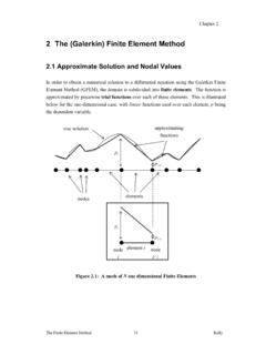
5 As an example, consider the 1-D heat equation for a uniform rod subject to some initial temperature distribution and whose ends are submerged in an ice bath. Figure graphically displays such a system. Figure Graphical representation of a uniform rod of length L subject to some initial temperature distribution u0(x) and whose ends are submerged in ice baths. The governing dynamical equation describing the conduction of heat along the rod in time is given by: x=0x=LICE ICE u(x,0) = u0(x) x 46 Lxforttxuxtxux = 0),(),(2 ( ) subject to the initial temperature distribution )()0,(0xuxu= ( ) and constrained by the following boundary conditions imposed by the ice baths: 0),(),0(==tLutu.

6 ( ) The term2 in Equation is known as the thermal diffusivity of the rod and is defined as s =2, ( ) where is the thermal conductivity, is the density, and s is the specific heat of the rod. Equations combine to define the strong form of the governing dynamics. Physically, Equations state that the heat flux is proportional to the temperature gradient along the rod. The boundary conditions (Equation ) are said to be homogeneous since they are specified as being equal to zero on both ends of the rod. Had the problem been defined with non-zero terms at each end, the boundary conditions would be referred to as non-homogeneous.

7 Without actually solving Equation , we know that the solution, u(x,t), to the problem will require two spatial derivatives, and it will have to satisfy the homogeneous boundary conditions while being subject to an initial temperature distribution. Thus, in more general terms, the strong solution to Equation satisfies the differential equation and 47boundary conditions exactly and must be as smooth (number of continuous derivatives) as required by the differential equation. The fact that the strong solution must be as smooth as required by the strong form of the differential equation is an immediate downfall of the strong form.

8 If the system under analysis consists of varying geometry or material properties, then discontinuous functions will enter into the equations of motion and the issue of differentiability can become immediately apparent. To avoid such difficulties, we can change the strong form of the governing dynamics into a weak or weighted-integral formulation. If the weak form to a differential equation exists, then we can arrive at it through a series of steps. First, for convenience, rewrite Equation in a more compact form, namely []txxuu=2 , ( ) where the subscripts x and t refer to spatial and temporal partial derivatives, respectively.

9 Next, move all the expressions of the differential equation to one side, multiply through the entire equation by an arbitrary function g, called the weight or test function, and integrate over the domain = [0, L] of the system: []()002= + Ltxxdxuug . ( ) Reddy (1993) refers to Equation as the weighted-integral or weighted-residual statement, and it is equivalent to the original system dynamics, Equation Another way of stating Equation is when the solution u(x,t) is exact, the solution to Equation is trivial. But, when we put an approximation in for u(x,t), there will be a non-zero value left in the parenthetical of Equation 6.

10 Mathematically, [Equation ] is a statement that the error in the differential equation (due to the approximation of the solution) is zero in the weighted-integral sense (Reddy, 1993). 48 Since we are seeking an approximation to the dynamics given by Equation , the weighted-integral form gives us a means to obtain N linearly independent equations to solve for the coefficients ci in the approximation == NiiiNxtctxutxu1)()(),(),( . ( ) Note that the weighted-integral form of the dynamic equation is not subject to any boundary conditions. The boundary conditions will come into play subsequently.