Transcription of CHAPTER 3 Frequency Response of Basic BJT and MOSFET ...
1 CHAPTER 3 Frequency Response of Basic BJT and MOSFET Amplifiers (Review materials in Appendices III and V) In this CHAPTER you will learn about the general form of the Frequency domain transfer function of an amplifier. You will learn to analyze the amplifier equivalent circuit and determine the critical frequencies that limit the Response at low and high frequencies. You will learn some special techniques to determine these frequencies. BJT and MOSFET amplifiers will be considered. You will also learn the concepts that are pursued to design a wide band width amplifier. Following topics will be considered. Review of Bode plot technique. Ways to write the transfer ( , gain) functions to show Frequency dependence. Band-width limiting at low frequencies ( , DC to fL).
2 Determination of lower band cut-off Frequency for a single-stage amplifier short circuit time constant technique. Band-width limiting at high frequencies for a single-stage amplifier. Determination of upper band cut-off Frequency - several alternative techniques. Frequency Response of a single device (BJT, MOSFET ). Concepts related to wide-band amplifier design BJT and MOSFET examples. A short review on Bode plot technique Example: Produce the Bode plots for the magnitude and phase of the transfer function 2510()(1/ 1 0 ) (1/ 1 0 )sTsss , for frequencies between 1 rad/sec to 106 rad/sec. We first observe that the function has zeros and poles in the numerical sequence 0 (zero), 102 (pole), and 105 (pole). Further at =1 rad/sec , lot less than the first pole (at =102 rad/sec), () 10 Tss.
3 Hence the first portion of the plot will follow the asymptotic line rising at 6 dB/octave, or 20 dB/decade, in the neighborhood of =1 rad/sec. The magnitude of T(s) in decibels will be approximately 20 dB at = 1 rad/sec. The second asymptotic line will commence at the pole of =102 rad/sec, running at -6 dB/octave slope relative to the previous asymptote. Thus the overall asymptote will be a line of slope zero, , a line parallel to the - axis. The third asymptote will commence at the pole =105 rad/sec, running at -6 dB/Octave slope relative to the previous asymptote. The overall asymptote will be a line dropping off at -6 dB/octave beginning from =105 rad/sec. Since we have covered all the poles and zeros, we need not work on sketching any further asymptotes.
4 The three asymptotic lines are now sketched as shown in figure Figure : The asymptotic line plots for the T(s). The actual plot will follow the asymptotic lines being 3 dB below the first corner point ( ,at =100) , 57 dB ,and 3 dB below the second corner point ( , =10^5), 57 dB. In between the two corner point the plot will approach the asymptotic line of constant value 60 dB. The magnitude plot is shown in figure Asymptote lines Figure :Bode magnitude plot for T(s) For phase plot, we note that the s in the numerator will give a constant phase shift of +90o degrees (since 0,sjj angle: 11tan ( / 0)tan ( )90o ), while the terms in the denominator will produce angles of 12tan ( /10 ) , and 15tan ( /10 ) respectively.
5 The total phase angle will then be: 12 15( ) 90tan ( /10 ) tan ( /10 )o ( ) Thus at low Frequency (<< 100 rad/sec), the phase angle will be close to 90o. Near the pole Frequency =100, a -45o will be added due to the ploe at making the phase angle to be close to +45o. The phase angle will progressively decrease, because of the first two terms in ( ). Near the second pole =105, the phase angle will approach 15 215 5( ) 90tan (10 /10 ) tan (10 /10 ) 909045oooo , -45o degrees. (The student in encouraged to draw the curve) Simplified form of the gain function of an amplifier revealing the Frequency Response limitation Magnitude plot (heavier line) Gain function at low frequencies Electronic amplifiers are limited in Frequency Response in that the Response magnitude falls off from a constant mid-band value to lower values both at frequencies below and above an intermediate range (the mid-band) of frequencies.
6 A typical Frequency Response curve of an amplifier system appears as in Figure : Typical Frequency Response function magnitude plot for an electronic amplifier Using the concepts of Bode magnitude plot technique, we can approximate the low- Frequency portion of the sketch above by an expression of the form asKssTL )(, or saKsTL/1)( . In this K and a are constants and s=j , where is the (physical, , measurable) angular Frequency (in rad/sec). In either case, when the signal Frequency is very much smaller than the pole Frequency a , the Response TL(s) takes the form aKs/. This function increases progressively with the Frequency js , following the asymptotic line with a slope of +6 dB per octave.
7 At the pole Frequency a , the Response will be 3 dB below the previous asymptotic line, and henceforth follow an asymptotic line of slope (-6+6=0) of zero dB/ octave. Thus TL(s) will remain constant with Frequency , assuming the mid-band value. Note that TL(s) is a first order function in s (a single time-constant function). The Frequency at which the magnitude plot reaches 3 dB below the mid-band ( , the flat portion of the magnitude Response curve) gain value is known as the -3 dB Frequency of the gain function. For the low- Frequency segment ( , TL(s)) of the magnitude plot this will be designated by fL (or L =2 fL). In a practical case the function TL(s) may have several poles and zeros at low frequencies.
8 The pole which is closest to the flat mid-band value is known as the low Frequency dominant pole of the system. Thus it is the pole of highest magnitude among all the poles and zeros at low frequencies. Numerically the dominant pole differs from the -3 dB Frequency . But for simplicity, one can approximate dominant pole to be of same value as the -3dB Frequency . The -3dB Frequency at low frequencies is also sometimes referred to as the lower cut-off Frequency of the amplifier system. The Frequency Response limitation at low Frequency occurs because of coupling and by-pass capacitors used in the amplifier circuit. For single-stage amplifiers, , CE, ,CG amplifiers these capacitors come in series with the signal path ( , they form a loop in the signal path), and hence impedes the flow of signal coupled to the internal nodes ( , BE nodes of the BJT, GS nodes of the MOSFET ) of the active device.
9 The students can convince themselves by considering the simple illustration presented in figure sigRBR r vSv1C vgm)||(1)||(11 BsigBSRrRsCsCRrvv asKsvvsTS )(1 Figure : Illustrating the formation of s zero in the voltage transfer function because of a capacitor in the signal loop. The controlling voltage v for the VCCS has a zero because of the presence of C1. Gain function at high frequencies A similar scenario exists for the Response at high frequencies. By considering the graph in at frequencies beyond ( , higher than) the mid-band segment, we can propose the form of the Response function as: bsKsTH )(. K and b are constants. Other alternative forms are: bsbKsToH )(, or bsKsToH/1)( . Note that in all cases, for frequencies << the pole Frequency b , the Response function assumes a constant value ( , the mid-band Response ).
10 For TH(s), which is a first-order function, the Frequency b becomes the -3db Frequency for high Frequency Response , or the upper cut-off Frequency . When there are several poles and zeros in the high Frequency range, the pole with the smallest magnitude and hence closest to the mid-band Response zone is referred to as the high Frequency dominant pole. Again, numerically the high Frequency dominant pole will be different from the upper cut-off Frequency . But in most practical cases, the difference is small. In case the high Frequency Response has several poles and zeros, one can formulate the function as 1212(1/) (1/) ..()(1/) (1/) ..zzHppssTsss ( ) In an integrated circuit scenario coupling or by-pass capacitors are absent.