Transcription of Chapter 3 Interpolation - MathWorks
1 Chapter 3 InterpolationInterpolation is the process of defining a function that takes on specified values atspecified points. This Chapter concentrates on two closely related interpolants: thepiecewise cubic spline and the shape-preserving piecewise cubic named pchip. The Interpolating PolynomialWe all know that two points determine a straight line. More precisely, any twopoints in the plane, (x1,y1) and (x2,y2), withx1 =x2, determine a unique first-degree polynomial inxwhose graph passes through the two points. There aremany different formulas for the polynomial, but they all lead to the same straightline generalizes to more than two points. Givennpoints in the plane,(xk,yk),k= 1,..,n, with distinctxk s, there is a unique polynomial inxof degreeless thannwhose graph passes through the points. It is easiest to remember thatn,the number of data points, is also the number of coefficients, although some of theleading coefficients might be zero, so the degree might actually be less thann , there are many different formulas for the polynomial, but they all define thesame polynomial is called theinterpolatingpolynomial because it exactly re-produces the given data:P(xk) =yk,k= 1.
2 , , we examine other polynomials, of lower degree, that only approximate thedata. They arenotinterpolating most compact representation of the interpolating polynomial is theLa-grangeformP(x) = k j =kx xjxk xj 16, 201312 Chapter 3. InterpolationThere arenterms in the sum andn 1 terms in each product, so this expressiondefines a polynomial of degree at mostn 1. IfP(x) is evaluated atx=xk, all theproducts except thekth are zero. Furthermore, thekth product is equal to one, sothe sum is equal toykand the Interpolation conditions are example, consider the following data = 0:3;y = [-5 -6 -1 16];The commanddisp([x; y])displays0 1 2 3-5 -6 -1 16 The Lagrangian form of the polynomial interpolating these data isP(x) =(x 1)(x 2)(x 3)( 6)( 5) +x(x 2)(x 3)(2)( 6)+x(x 1)(x 3)( 2)( 1) +x(x 1)(x 2)(6)(16).We can see that each term is of degree three, so the entire sum has degree atmost three. Because the leading term does not vanish, the degree is actually , if we plug inx= 0,1,2, or 3, three of the terms vanish and the fourthproduces the corresponding value from the data are not usually represented in their Lagrangian form.
3 More fre-quently, they are written as something likex3 2x simple powers ofxare calledmonomials, and this form of a polynomial is saidto be using thepower coefficients of an interpolating polynomial using its power form,P(x) =c1xn 1+c2xn 2+ +cn 1x+cn,can, in principle, be computed by solving a system of simultaneous linear equations xn 11xn 21 x11xn 12xn 22 x21 1xn 1nxn 2n xn1 = .The matrixVof this linear system is known as aVandermondematrix. Itselements arevk;j=xn The Interpolating Polynomial3 The columns of a Vandermonde matrix are sometimes written in the opposite order,but polynomial coefficient vectors inMatlabalways have the highest power Vandermonde matrices. For our ex-ample data set,V = vander(x)generatesV =0 0 0 11 1 1 18 4 2 127 9 3 1 Thenc = V\y'computes the = fact, the example data were generated from the polynomialx3 2x asks you to show that Vandermonde matrices are nonsingular ifthe pointsxkare distinct.
4 But Exercise asks you to show that a Vandermondematrix can be very badly conditioned. Consequently, using the power form andthe Vandermonde matrix is a satisfactory technique for problems involving a fewwell-spaced and well-scaled data points. But as a general-purpose approach, it this Chapter , we describe severalMatlabfunctions that implement variousinterpolation algorithms. All of them have the calling sequencev =interp(x,y,u)The first two input arguments,xandy, are vectors of the same length that definethe interpolating points. The third input argument,u, is a vector of points wherethe function is to be evaluated. The outputvis the same length asuand haselementsv(k)=interp(x,y,u(k))Our first such Interpolation function,polyinterp, is based on the Lagrangeform. The code usesMatlabarray operations to evaluate the polynomial at allthe components 3. Interpolationfunction v = polyinterp(x,y,u)n = length(x);v = zeros(size(u));for k = 1:nw = ones(size(u));for j = [1:k-1 k+1:n]w = (u-x(j)).
5 /(x(k)-x(j)).*w;endv = v + w*y(k);endTo illustratepolyinterp, create a vector of densely spaced evaluation = :.01 ;Thenv = polyinterp(x,y,u);plot(x,y,'o',u,v,'-')c reates Figure 10 50510152025 Figure also works correctly with symbolic variables. Forexample, createsymx = sym('x')Then evaluate and display the symbolic form of the interpolating polynomial The Interpolating Polynomial5P = polyinterp(x,y,symx)pretty(P)which producesP =(x*(x - 1)*(x - 3))/2 + 5*(x/2 - 1)*(x/3 - 1)*(x - 1) +(16*x*(x/2 - 1/2)*(x - 2))/3 - 6*x*(x/2 - 3/2)*(x - 2)/ x\16 x | - - 1/2 | (x - 2)x (x - 1) (x - 3) / x \ / x \\ 2/----------------- + 5 | - - 1 | | - - 1 | (x - 1) + ------------------------2\ 2 / \ 3 /3/ x\- 6 x | - - 3/2 | (x - 2)\ 2/This expression is a rearrangement of the Lagrange form of the interpolating poly-nomial. Simplifying the Lagrange form withP = simplify(P)changesPto the power formP =x^3 - 2*x - 5 Here is another example, with a data set that is used by the other methodsin this = 1:6;y = [16 18 21 17 15 12];disp([x; y])u =.
6 75:.05 ;v = polyinterp(x,y,u);plot(x,y,'o',u,v,'r-') ;produces1 2 3 4 5 616 18 21 17 15 12and Figure in this example, with only six nicely spaced points, we can begin tosee the primary difficulty with full-degree polynomial Interpolation . In betweenthe data points, especially in the first and last subintervals, the function showsexcessive variation. It overshoots the changes in the data values. As a result, full-degree polynomial Interpolation is hardly ever used for data and curve fitting. Itsprimary application is in the derivation of other numerical 3. Interpolation12345610121416182022 Full degree polynomial interpolationFigure polynomial Piecewise Linear InterpolationYou can create a simple picture of the data set from the last section by plottingthe data twice, once with circles at the data points and once with straight linesconnecting the points. The following statements produce Figure = 1:6;y = [16 18 21 17 15 12];plot(x,y,'o',x,y,'-');To generate the lines, theMatlabgraphics routines usepiecewise linearin-terpolation.
7 The algorithm sets the stage for more sophisticated algorithms. Threequantities are involved. Theinterval indexkmust be determined so thatxk x<xk+ variable,s, is given bys=x divided differenceis k=yk+1 ykxk+1 these quantities in hand, the interpolant isL(x) =yk+ (x xk)yk+1 ykxk+1 Piecewise Linear Interpolation712345610121416182022 Piecewise linear interpolationFigure linear +s is clearly a linear function that passes through (xk,yk) and (xk+1,yk+1).The pointsxkare sometimes calledbreakpointsorbreaks. The piecewise linearinterpolantL(x) is a continuous function ofx, but its first derivative,L (x), is notcontinuous. The derivative has a constant value, k, on each subinterval and jumpsat the linear Interpolation is implemented The inputucan be a vector of points where the interpolant is to be evaluated, so the indexkisactually a vector of indices. Read this code carefully to see howkis v = piecelin(x,y,u)%PIECELIN Piecewise linear v = piecelin(x,y,u) finds the piecewise linear L(x)% with L(x(j)) = y(j) and returns v(k) = L(u(k)).
8 % First divided differencedelta = diff(y)./diff(x);% Find subinterval indices k so that x(k) <= u < x(k+1)n = length(x);k = ones(size(u));for j = 2:n-18 Chapter 3. Interpolationk(x(j) <= u) = j;end% Evaluate interpolants = u - x(k);v = y(k) + s.*delta(k); Piecewise Cubic Hermite InterpolationMany of the most effective Interpolation techniques are based on piecewise cubicpolynomials. Lethkdenote the length of thekth subinterval:hk=xk+1 the first divided difference, k, is given by k=yk+1 the slope of the interpolant atxk:dk=P (xk).For the piecewise linear interpolant,dk= k 1or k, but this is not necessarily truefor higher order the following function on the intervalxk x xk+1, expressed interms of local variabless=x xkandh=hk:P(x) =3hs2 2s3h3yk+1+h3 3hs2+ 2s3h3yk+s2(s h)h2dk+1+s(s h) is a cubic polynomial ins, and hence inx, that satisfies four interpolationconditions, two on function values and two on the possibly unknown derivativevalues:P(xk) =yk,P(xk+1) =yk+1,P (xk) =dk,P (xk+1) =dk+ that satisfy Interpolation conditions on derivatives are known asHermiteorosculatoryinterpolants, because of the higher order contact at the interpolationsites.
9 ( Osculari means to kiss in Latin.)If we happen to know both function values and first derivative values at aset of data points, then piecewise cubic Hermite Interpolation can reproduce thosedata. But if we are not given the derivative values, we need to define the slopesdksomehow. Of the many possible ways to do this, we will describe two, Shape-Preserving Piecewise Shape-Preserving Piecewise CubicThe acronympchipabbreviates piecewise cubic Hermite interpolating polyno-mial. Although it is fun to say, the name does not specify which of the manypossible interpolants is actually being used. In fact, spline interpolants are alsopiecewise cubic Hermite interpolating polynomials, but with different slopes. Ourparticularpchipis a shape-preserving, visually pleasing interpolant that was in-troduced intoMatlabfairly recently. It is based on an old Fortran program byFritsch and Carlson [2] that is described by Kahaner, Moler, and Nash [3]. shows howpchipinterpolates our sample preserving Hermite interpolationFigure piecewise cubic Hermite key idea is to determine the slopesdkso that the function values do notovershoot the data values, at least locally.
10 If kand k 1have opposite signs or ifeither of them is zero, thenxkis a discrete local minimum or maximum, so we setdk= is illustrated in the first half of Figure The lower solid line is the piecewiselinear interpolant. Its slopes on either side of the breakpoint in the center haveopposite signs. Consequently, the dashed line has slope zero. The curved line isthe shape-preserving interpolant, formed from two different cubics. The two cubicsinterpolate the center value and their derivatives are both zero there. But there isa jump in the second derivative at the kand k 1have the same sign and the two intervals have the same length,10 Chapter 3. Interpolationthendkis taken to be the harmonic mean of the two discrete slopes:1dk=12(1 k 1+1 k).In other words, at the breakpoint, the reciprocal slope of the Hermite interpolantis the average of the reciprocal slopes of the piecewise linear interpolant on eitherside. This is shown in the other half of Figure At the breakpoint, the reciprocalslope of the piecewise linear interpolant changes from 1 to 5.


![The Delta Sequence - - - [n]](/cache/preview/4/5/f/4/3/f/1/e/thumb-45f43f1eaf2ef1960b4bc76c800b38e3.jpg)