Transcription of Chapter 4
1 Chapter 4 Dynamical Equations for FlightVehiclesThese notes provide a systematic background of the derivation of the equations of motionfor a flight vehicle, and their linearization. The relationship between dimensional stabilityderivatives and dimensionless aerodynamic coefficients is presented, and the principalcontributions to all important stability derivatives for flight vehicles having left/rightsymmetry are Basic Equations of MotionThe equations of motion for a flight vehicle usually are written in a body-fixed coordinate is convenient to choose the vehicle center of mass as the origin for this system, and the orientationof the (right-handed) system of coordinate axes is chosen byconvention so that, as illustrated inFig. : thex-axis lies in the symmetry plane of the vehicle1and points forward; thez-axis lies in the symmetry plane of the vehicle, is perpendicular to thex-axis, and pointsdown; they-axis is perpendicular to the symmetry plane of the vehicle and points out the right precise orientation of thex-axis depends on the application; the two most common choices are: to choose the orientation of thex-axis so that the product of inertiaIxz=Zmxzdm= 01 Almost all flight vehicles have bi-lateral (or, left/right)symmetry, and most flight dynamics analyses take advan-tage of this 4.
2 DYNAMICAL EQUATIONS FOR FLIGHT VEHICLESThe other products of inertia,IxyandIyz, are automatically zero by vehicle symmetry. Whenall products of inertia are equal to zero, the axes are said tobeprincipal axes. to choose the orientation of thex-axis so that it is parallel to the velocity vector for an initialequilibrium state. Such axes are calledstability choice of principal axes simplifies the moment equations, and requires determination of only oneset of moments of inertia for the vehicle at the cost of complicating theX- andZ-force equationsbecause the axes will not, in general, be aligned with the lift and drag forces in the equilibrium choice of stability axes ensures that the lift and drag forces in the equilibrium state are alignedwith theZandXaxes, at the cost of additional complexity in the moment equations and the needto re-evaluate the inertial properties of the vehicle (Ix,Iz, andIxz)
3 For each new equilibrium Force EquationsThe equations of motion for the vehicle can be developed by writing Newton s second law for eachdifferential element of mass in the vehicle,d~F=~adm( )then integrating over the entire vehicle. When working out the acceleration of each mass element, wemust take into account the contributions to its velocity from both linear velocities (u, v, w) in each ofthe coordinate directions as well as the~ ~rcontributions due to the rotation rates (p, q, r) aboutthe axes. Thus, the time rates of change of the coordinates inan inertial frame instantaneouslycoincident with the body axes are x=u+qz ry y=v+rx pz z=w+py qx( ) xzyFigure : Body axis system with origin at center of gravityof a flight vehicle. Thex-zplane liesin vehicle symmetry plane, andy-axis points out right BASIC EQUATIONS OF MOTION39and the corresponding accelerations are given by x=ddt(u+qz ry) y=ddt(v+rx pz) z=ddt(w+py qx)( )or x= u+ qz+q(w+py qx) ry r(v+rx pz) y= v+ rx+r(u+qz ry) pz p(w+py qx) z= w+ py+p(v+rx pz) qx q(u+qz ry)( )Thus, the net product of mass times acceleration for the entire vehicle ism~a=Zm{[ u+ qz+q(w+py qx) ry r(v+rx pz)] +[ v+ rx+r(u+qz ry) pz p(w+py qx)] +[ w+ py+p(v+rx pz) qx q(u+qz ry)] kodm( )Now, the velocities and accelerations, both linear and angular, are constant during the integrationover the vehicle coordinates, so the individual terms in Eq.}
4 ( ) consist of integrals of the formZmdm=mwhich integrates to the vehicle massm, andZmxdm=Zmydm=Zmzdm= 0,( )which are all identically zero since the origin of the coordinate system is at the vehicle center ofmass. Thus, Eq. ( ) simplifies tom~a=mh( u+qw rv) + ( v+ru pw) + ( w+pv qu) ki( )To write the equation corresponding to Newton s Second Law,we simply need to set Eq. ( ) equalto the net external force acting on the vehicle. This force isthe sum of the aerodynamic (includingpropulsive) forces and those due to order to express the gravitational force acting on the vehicle in the body axis system, we needto characterize the orientation of the body axis system withrespect to the gravity vector. Thisorientation can be specified using theEuler anglesof the body axis system with respect to aninertial system (xf, yf, zf), where the inertial system is oriented such that thezfaxis points down ( , is parallel to the gravity vector~g); thexfaxis points North; and theyfaxis completes the right-handed system and, therefore, points 4.
5 DYNAMICAL EQUATIONS FOR FLIGHT VEHICLESxxy1fz , zf1f y1x1y1 xzz212, y2xz2 , x2zyy2(a)(b)(c)Figure : The Euler angles , , and determine the orientation of the body axes of a flightvehicle. (a) Yaw rotation aboutz-axis, nose right; (b) Pitch rotation abouty-axis, nose up; (c) Rollrotation aboutx-axis, right wing orientation of the body axis system is specified by starting with the inertial system, then,inthe following orderperforming:1. a positive rotation about thezfaxis through the heading angle to produce the (x1, y1, z1)system; then2. a positive rotation about they1axis through the pitch angle to produce the (x2, y2, z2)system; and, finally3. a positive rotation about thex2axis through the bank angle to produce the (x, y, z) , if we imagine the vehicle oriented initially with itsz-axis pointing down and heading North,its final orientation is achieved by rotating through the heading angle , then pitching up throughangle , then rolling through angle.
6 This sequence of rotations in sketched in Fig. we are interested only in the orientation of the gravity vector in the body axis system, we canignore the first , we need consider only the second rotation, in which thecomponentsof any vector transform as x2y2z2 = cos 0 sin 0 10sin 0 cos xfyfzf ( )and the third rotation, in which the components transform as xyz = 1000 cos sin 0 sin cos x2y2z2 ( )2If we are interested in determining where the vehicle is going say, we are planning a flight path to get us fromNew York to London, we certainly are interested in the heading, but this is not really an issue as far as analysis ofthe stability and controllability of the vehicle are BASIC EQUATIONS OF MOTION41 Thus, the rotation matrix from the inertial frame to the bodyfixed system is seen to be xyz = 1000 cos sin 0 sin cos cos 0 sin 0 10sin 0 cos xfyfzf = cos 0 sin sin sin cos cos sin sin cos sin cos cos xfyfzf ( )
7 The components of the gravitational acceleration in the body-fixed system are, therefore, gxgygz = cos 0 sin sin sin cos cos sin sin cos sin cos cos 00g0 =g0 sin cos sin cos cos ( )The force equations can thus be written as XYZ +mg0 sin cos sin cos cos =m u+qw rv v+ru pw w+pv qu ( )where (X, Y, Z) are the components of the net aerodynamic and propulsive forces acting on thevehicle, which will be characterized in subsequent Moment EquationsThe vector form of the equation relating the net torque to therate of change of angular momentumis~G= LMN =Zm(~r ~a) dm( )where (L, M, N) are the components about the (x, y, z) body axes, respectively, of the net aerody-namic and propulsive moments acting on the vehicle. Note that there is no net moment due to thegravitational forces, since the origin of the body-axis system has been chosen at the center of massof the vehicle.
8 The components of Eq.( ) can be written asL=Zm(y z z y) dmM=Zm(z x x z) dmN=Zm(x y y x) dm( )where x, y, and zare the net accelerations in an inertial system instantaneously coincident with thebody axis system, as given in Eqs. ( ).When Eqs. ( ) are substituted into Eqs. ( ), the terms in the resulting integrals are eitherlinear or quadratic in the coordinates. Since the origin of the body-axis system is at the vehicle ,42 Chapter 4. DYNAMICAL EQUATIONS FOR FLIGHT VEHICLESEqs. ( ) apply and the linear terms integrate to zero. The quadratic terms can be expressed interms of themoments of inertiaIx=Zm y2+z2 dmIy=Zm z2+x2 dmIz=Zm x2+y2 dm( )and theproduct of inertiaIxz=Zmxzdm( )Note that the products of inertiaIxy=Iyz= 0, since they-axis is perpendicular to the assumedplane of symmetry of the ( ) can then be written asL=Ix p+ (Iz Iy)qr Ixz(pq+ r)M=Iy q+ (Ix Iz)rp Ixz p2 r2 N=Iz r+ (Iy Ix)pq Ixz(qr p)( )Note that if principal axes are used, so thatIxz 0, Eqs.
9 ( ) simplify toL=Ix p+ (Iz Iy)qrM=Iy q+ (Ix Iz)rpN=Iz r+ (Iy Ix)pq( ) Linearized Equations of MotionThe equations developed in the preceding section completely describe the motion of a flight vehicle,subject to the prescribed aerodynamic (and propulsive) forces and moments. These equations arenonlinearandcoupled, however, and generally can be solved only numerically, yielding relatively lit-tle insight into the dependence of the stability and controllability of the vehicle on basic aerodynamicparameters of the great deal, however, can be learned by studyinglinearapproximations to these equations. Inthis approach, we analyze the solutions to the equations describingsmall perturbationsabout anequilibrium flight condition. The greatest simplification of the equations arises when the equilibriumcondition is chosen to correspond to alongitudinalequilibrium, in which the velocity and gravityvectors lie in the plane of symmetry of the vehicle; the most common choice corresponds to unaccel-erated flight , to level, unaccelerated flight, or to steady climbing (or descending) flight.
10 Sucha linear analysis has been remarkably successful in flight dynamics applications,3primarily because:3 This statement should be interpreted in the context of the difficulty of applying similar linear analyses to othersituations , to road vehicle dynamics, in which the stability derivatives associated with tire forces are LINEARIZED EQUATIONS OF MOTION431. Over a fairly broad range of flight conditions of practicalimportance, the aerodynamic forcesand moments are well-approximated as linear functions of the state variables; and2. Normal flight situations correspond to relatively small variations in the state variables; in fact,relatively small disturbances in the state variables can lead to significant accelerations, , toflight of considerable violence, which we normally want to , we should emphasize the caveat that these linear analyses are not good approximations insome cases particularly for spinning or post-stall flight , we will consider1.