Transcription of Chapter 4 Model Adequacy Checking - IIT Kanpur
1 regression Analysis | Chapter 4 | Model Adequacy Checking | Shalabh, IIT Kanpur 1 1 1 Chapter 4 Model Adequacy Checking The fitting of linear regression Model , estimation of parameters testing of hypothesis properties of the estimator are based on following major assumptions: 1. The relationship between the study variable and explanatory variables is linear, atleast approximately. 2. The error term has zero mean. 3. The error term has constant variance. 4. The errors are uncorrelated. 5. The errors are normally distributed. The validity of these assumption is needed for the results to be meaningful. If these assumptions are violated, the result can be incorrect and may have serious consequences.
2 If these departures are small, the final result may not be changed significantly. But if the departures are large, the Model obtained may become unstable in the sense that a different sample could lead to a entirely different Model with opposite conclusions. So such underlying assumptions have to be verified before attempting to regression modeling. Such information is not available from the summary statistic such as t-statistic, F-statistic or coefficient of determination. One important point to keep in mind is that these assumptions are for the population and we work only with a sample. So the main issue is to take a decision about the population on the basis of a sample of data.
3 Several diagnostic methods to check the violation of regression assumption are based on the study of Model residuals with the help of various types of graphics. Checking of linear relationship between study and explanatory variables 1. Case of one explanatory variable If there is only one explanatory variable in the Model , then it is easy to check the existence of linear relationship between y and X by scatter diagram of the available data. If the scatter diagram shows a linear trend, it indicates that the relationship between y and X is linear. If the trend is not linear, then it indicates that the relationship between y and X is nonlinear.
4 For example, the following figure indicates a linear trend regression Analysis | Chapter 4 | Model Adequacy Checking | Shalabh, IIT Kanpur 2 2 2 whereas the following figure indicates a nonlinear trend: 2. Case of more than one explanatory variables To check the assumption of linearity between study variable and explanatory variables, the scatter plot matrix of the data can be used. A scatterplot matrix is a two dimensional array of two dimension plots where each form contains a scatter diagram except for the diagonal. Thus, each plot sheds some light on the relationship between a pair of variables. It gives more information than the correlation coefficient between each pair of variables because it gives a sense of linearity or nonlinearity of the relationship and some regression Analysis | Chapter 4 | Model Adequacy Checking | Shalabh, IIT Kanpur 3 3 3 awareness of how the individual data points are arranged over the region.
5 It is a scatter diagram of 1( versus ),yX 2( versus ), , ( versus )kyX. Another option to present the scatterplot is - present the scatterplots in the upper triangular part of plot matrix. - Mention the corresponding correlation coefficients in the lower triangular part of the matrix. Suppose there are only two explanatory variables and the Model is 112 2,yXX =++ then the scatterplot matrix looks like as follows. Such arrangement helps in examining of plot and corresponding correlation coefficient together. The pairwise correlation coefficient should always be interpreted in conjunction with the corresponding scatter plots because - the correlation coefficient measures only the linear relationship and - the correlation coefficient is non-robust, , its value can be substantially influenced by one or two observations in the data.
6 regression Analysis | Chapter 4 | Model Adequacy Checking | Shalabh, IIT Kanpur 4 4 4 The presence of linear patterns is reassuring but absence of such patterns does not imply that linear Model is incorrect. Most of the statistical software provide the option for creating the scatterplot matrix. The view of all the plots provides an indication that a multiple linear regression Model may provide a reasonable fit to the data. It is to be kept is mind that we get only the information on pairs of variables through the scatterplot of 1( versus ),yX 2( versus ), , ( versus )kyX whereas the assumption of linearity is between y and jointly with (12.)
7 ,).kXX X If some of the explanatory variables are themselves interrelated, then these scatter diagrams can be misleading. Some other methods of sorting out the relationships between several explanatory variables and a study variable are used. Residual analysis The residual is defined as the difference between the observed and fitted value of study variable. The thi residual is defined as ~,1, 2,..,iiiiie y y y yin= = = where iy is an observation and iy is the corresponding fitted value. Residual can be viewed as the deviation between the data and the fit. So it is also a measure of the variability in the response variable that is not explained by the regression Model .
8 Residuals can be thought as the observed values of the Model errors. So it can be expected that if there is any departure from the assumptions on random errors, then it should be shown up by the residual. Analysis of residual helps is finding the Model inadequacies. Assuming that the regression coefficients in the Model yX = + are estimated by the OLSE, we find that: Residuals have zero mean as ()()()00iiii iiiiEeE y yE XXbXX = = + = + = Approximate average variance of residuals is estimated by regression Analysis | Chapter 4 | Model Adequacy Checking | Shalabh, IIT Kanpur 5 5 5 2211ee()nniiiirsrseeeSSMS nknk nk== ===.
9 Residuals are not independent as the n residuals have only nk degrees of freedom. The nonindependence of the residuals has little effect on their use for Model Adequacy Checking as long as n is not small relative to .k Methods for scaling residuals Sometimes it is easier to work with scaled residuals. We discuss four methods for scaling the residuals . 1. Standardized residuals: The residuals are standardized based on the concept of residual minus its mean and divided by its standard deviation. Since () 0iEe= and ersMS estimates the approximate average variance, so logically the scaling of residual is e,1, 2,..,iirsedinMS== is called as standardized residual for which () 0( ) d= So a large value of ( 3,id> say) potentially indicates an outlier.
10 2. Studentized residuals The standardized residuals use the approximate variance of ie as ersMS. The studentized residuals use the exact variance of ie. We first find the variance of ie. In the Model yX = +, the OLSE of is 1(') 'b XX Xy = and the residual vector is regression Analysis | Chapter 4 | Model Adequacy Checking | Shalabh, IIT Kanpur 6 6 6 1 ()where(' )' ()() () () () e yyy Xby HyI H yH XXX XI HXXHXIHX XIHIHH = = = = == += + = + = = Thus eHyH = =, so residuals are the same linear transformation of y and . The covariance matrix of residuals is 22()( )()()Ve VHHVHHIH ==== and 2().