Transcription of Chapter 4: Quantitative genetics I: Genetic …
1 Conner and Hartl p. 4-1 From: Conner, J. and D. Hartl, A Primer of Ecological genetics . In prep. for SinauerChapter 4: Quantitative genetics I: Genetic Mendelian basis of continuous traitsThe previous chapters have focused on the population genetics of single loci with only twoalleles. If a large majority of variation in a phenotypic trait is determined by one locus, the resultis a visible polymorphism like Mendel s pea traits or flower color in Delphinium ( Chapter 2).However, as noted in Chapter 2, most phenotypic traits do not fall into distinct categories, butrather are continuously distributed. Examples of continuously distributed traits are shown inFigure These traits are called Quantitative or metric traits because they need to bemeasured, not just scored as round or wrinkled or blue or white.
2 In classical or statisticalquantitative genetics , the phenotypes of individuals of known Genetic relationship (usuallyparents and offspring or siblings) are measured, and the Genetic and environmental sources ofphenotypic variation are determined statistically. In the newer technique of Quantitative traitlocus (QTL) mapping, variation in Genetic markers that are scattered throughout the genome isstatistically related to phenotypic variation ( Chapter 5). Both techniques have strengths andweaknesses, and both are valuable for the study of natural populations. The key similarity is thatthey focus on continuously distributed phenotypic traits, whereas population genetics is muchmore concerned with discrete genotypes.
3 Population Genetic techniques are applied directly tophenotypes only in the rare cases where phenotypic variation is discrete, , visiblepolymorphisms. So for this Chapter and the next two, the emphasis is shifting from genotypes tophenotypic Continuously distributed traits. Shown are frequency distributions, where the height of each bar givesthe number of individuals with the trait value on the X-axis. Note that these traits are approximate a normaldistribution, which is common for many traits (sometimes statistical transformation is necessary). Data are from afield study of wild radish (Conner et al.)
4 In press).In population genetics the population is characterized with allele and genotype frequencies( Chapter 2). Because these are discrete, it is a simple matter to count individuals with eachNo. of individuals02040608010012014028 32 36 40 44 48 52 56 60 64 Flowering time (days) Length (mm)Conner and Hartl p. 4-2genotype and calculate the frequencies (proportions). We used F-statistics to understand howthis discrete variation is distributed within and among populations ( Chapter 3). With continuousphenotypic traits, in most cases the alleles that are present in the population or even the lociaffect the trait are unknown, so we need to use the statistical measures of mean and variance(and later covariance, Chapter 5) to characterize populations (Figure ).
5 This Chapter isdevoted to relating these two methods by showing how the means and variances are determinedby allele frequencies and the environment. In this way we will show how statistical quantitativegenetics is derived from Mendelian genetics , and set the stage for a discussion of QTL mappingin the next TraitFrequencyFigure Three normal distributions (idealized versions of real data such as that in Fig. ) illustratingmean and variance. The mean (single-headed arrows) is just the average phenotype in the population, and thevariance (double-headed arrows) is a measure of how variable the population is; in other words, the width of thedistribution.
6 Populations A and B have the same mean but different variances, while A and C have different meansbut the same variances. See Appendix 1 for the formulae for mean and phenotypic traits have this continuous distribution in spite of the fact that all geneticvariation is discrete, not continuous; for example, there are three distinct genotypes at a locuswith two alleles. This continuous distribution of most traits occurs for two reasons -- most traitshave more than one gene locus affecting them, and they are also affected, sometimes to a largedegree, by the environment. Remember that means, variances, and allele frequencies are allproperties of the population, but the first step in relating these is to discuss what determinesphenotypic value (P), which is simply the measurement of a given trait for a given example, the phenotypic value for the petal length of a plant in Fig.
7 Might be , and the same plant s for P for flowering time might be 44 days. The phenotypicvalue of an individual is determined by the individual s genotype and the environment, which wewill define as all non- Genetic effects on the phenotype:P = G + E ( )where G is the genotypic value and E is the environmental deviation. The genotypic value is thephenotype produced by a given genotype in the average environment, which means it can onlybe measured by replicating clones or highly inbred lines across environments, but it is a usefulconceptual tool for sexual species as well.
8 The graphs in Figure show the values of G foreach genotype with 2, 3, or six loci; this shows how adding loci makes the trait distribution morecontinuous even in the absence of any environmental and Hartl p. 4-3 Figure A hypothetical example (based on the real petal length data in Fig. ) showing genotypic values(along the X-axes). The three graphs show how increasing numbers of loci affecting a trait makes the traitdistribution more continuous in the absence of environmental deviations. In A, there are two loci with two alleleseach, which is the simplest case for a trait affected by more than one locus.
9 The loci act additively (no dominance orepistasis), so each capital letter allele adds mm of petal length over the aabb genotype, which has 5 mm table shows the frequency of each genotype under HWE and with p=q= for both loci, and the graph showsthe phenotypic distribution that results. B and C show the phenotypic distribution with 3 and 6 loci; in these caseseach capital letter allele adds 1 and mm respectively, keeping all other conditions the same as in factors usually vary continuously themselves think of temperature, rainfall,sunlight, prey availability, etc. Therefore, the environment causes the phenotypic valuesproduced by different individuals with the same genotype to deviate continuously from G; thesedeviations are the E term in eq.
10 In other words, the environmental deviation is thedifference between the phenotypic and genotypic values caused by the environment. Thesepoints illustrated in Figure , which depicts a set of hypothetical results from raising 12individuals with the AABB genotype from Figure each in a different environment. 3 loci1/161/43/80 FrequencyPetal Length (mm)GenotypeAABBAABbAAbbAaBBAaBbAabbaaBB aaBbaabb# LongAlleles432321210 Frequency1/161/81/161/81/41/81/161/81 6 lociPetal Length (mm)Conner and Hartl p. 4-4resulting distribution of environmental deviations reflects the most common assumptions inmodeling environmental effects, that is that E is normally distributed with mean = zero.