Transcription of Chapter 5 Boundary Value Problems
1 Chapter 5 Boundary Value ProblemsA Boundary Value problem for a given differential equation consists of finding a solution of thegiven differential equation subject to a given set of Boundary conditions . A Boundary conditionis a prescription some combinations of values of the unknownsolution and its derivatives at morethan one (a, b) Rbe an interval. Letp,q,r: (a, b) Rbe continuous this Chapter we consider the linear second orderequation given byy +p(x)y +q(x)y=r(x), a < x < b.( )Corresponding to ODE ( ), there are four important kinds of (linear) Boundary conditions . Theyare given byDirichlet or First kind :y(a) = 1, y(b) = 2,Neumann or Second kind :y (a) = 1, y (b) = 2,Robin or Third or Mixed kind : 1y(a) + 2y (a) = 1, 1y(b) + 2y (b) = 2,Periodic :y(a) =y(b), y (a) =y (b).Remark (On periodic Boundary condition)If the coefficients of ODE( )are periodicfunctions with periodl=b aand if is a solution of ODE( )(note that this solution existsonR), then defined by (x) = (x+l)is also a solution.
2 If satisfies the periodic boundaryconditions, then (a) = (a)and (a) = (a). Since solutions to IVP are unique in the presentcase, it must be that . In other words, is a periodic function of Value Problems do not behave as nicely as Initial Value Problems . For, there are BVPsfor which solutions do not exist; and even if a solution exists there might be many more. Thusexistence and uniqueness generally fail for BVPs. The following example illustrate all the the equationy +y= 0( )(i)The BVP for equation( )with Boundary conditionsy(0) = 1,y( 2) = 1has a uniquesolution. This solution is given bysinx+ cosx.(ii)The BVP for equation( )with Boundary conditionsy(0) = 1,y( ) = 1has no solutions.(iii)The BVP for equation( )with Boundary conditionsy(0) = 1,y(2 ) = 1has an infinitenumber of Adjoint forms, Lagrange Adjoint forms, Lagrange identityIn mathematical physics there are many important Boundary Value Problems corresponding tosecond order equations.
3 In the studies of vibrations of a membrane, vibrations of a structure onehas to solve a homogeneous Boundary Value problem for real frequencies (eigen values). As is well-known in the case of symmetric matrices that there are only real eigen values and correspondingeigen vectors form a basis for the underlying vector space and thereby all symmetric matricesare can be thought of as corresponding ODE versions ofsymmetric matrices, and they play an important role in mathematical us consider the equationL[y] l(x)y +p(x)y +q(x)y= 0, a < x < b.( )IntegratingzL[y] by parts fromatox, we haveZxazL[y]dx= (zl)y (zl) y+ (zp)y xa+Zxa (zl) (zp) + (zq) y dx.( )If we define the second order operatorL byL [z] (zl) (zp) + (zq) =l(x)z + (2l p)(x)z + (l p +q)(x)z= 0,( )then the equation ( ) becomesZxa zL[y] yL [z] dx= l(y z yz ) + (p l )y z xa.( )The operatorL is called theadjoint operatorcorresponding to the operatorL. It can be easilyverified that adjoint ofL isLitself.
4 IfLandL are the same, thenLis said to , the necessary and sufficient condition forLto be self-adjoint is thatp= 2l p,andq=l p +q,( )which is satisfied ifp=l .( )Thus ifLis self-adjoint, we haveL[y] l(x)y +p(x)y +q(x)y= l(x)y +q(x)y.( )A general operatorLmay not be self-adjoint but it can always be converted into a self-adjoint bysuitably multiplyingLwith a (self-adjointisation)The operatorh(x)L[y]is self-adjoint, wherehis given byh(x) =1l(x)exp Zxp(t)l(t)dt .( )In facth(x)L[y]is given byddx (x)dydx + (x)y= 0,( )where (x) = exp Zxp(t)l(t)dt , (x) =q(x)l(x)exp Zxp(t)l(t)dt .( )MA 417: Ordinary Differential EquationsSivaji Ganesh SistaChapter 5 : Boundary Value Problems43 Exercise (i)Prove that the self-adjoint form of the Legendre equation(1 x2)y 2xy +n(n+ 1)y= 0( )isddx (1 x2)dydx +n(n+ 1)y= 0.( )(ii)Prove that the self-adjoint form of the Bessel equationx2y +xy + (x2 2)y= 0( )isddx xdydx + x 2x y= 0.( )Lagrange identity, Green s identityDifferentiating both sides of equation ( ), we getLagrange identity: zL[y] yL [z] =ddx l(y z yz ) + (p l )y z.
5 ( )If we takex=bin the equation ( ), we getGreen s identity:Zba zL[y] yL [z] dx= l(y z yz ) + (p l )y z ba.( )IfLis self-adjoint, then Green s identity ( ) reduces toZba zL[y] yL[z] dx= l(y z yz ) ba,( )and Lagrange identity becomes zL[y] yL[z] =ddx l(y z yz ) .( ) Two-point Boundary Value problemIn this section we are going to set up the notations that we aregoing to use through out ourdiscussion of consider the linear nonhomogeneous second order in the self-adjoint form described (HBVP)Letf,qbe continuous function on the interval [a, b]. Letpbe a continuously differen-tiable and does not vanish on the interval [a, b]. Further assume thatp >0 on [a, b].The linear nonhomogeneous BVP in self-adjoint form then conists of solving the ODEL[y] ddx p(x)dydx +q(x)y=f(x),( )along with two Boundary conditions prescribed ataandbgiven byU1[y] a1y(a) +a2y (a) = 1,U2[y] b1y(b) +b2y (b) = 2,( )where 1and 2are given constants; and the constantsa1,a2,b1,b2satisfya21+a226= 0andb21+b226= Ganesh SistaMA 417: Ordinary Differential Two-point Boundary Value problemNote that the Boundary conditions are in the most general form, and they include the first threeconditions given at the beginning of our discussion on BVPs as special us introduce some nomenclature hypothesis(HBVP).
6 Anonhomogeneous Boundary Value problemconsists ofsolvingL[y] =f,U1[y] = 1,U2[y] = 2,( )for given constants 1and 2, and a given continuous functionfon the interval[a, b].Definition associatedhomogeneous Boundary Value problemis then given byL[y] = 0,U1[y] = 0,U2[y] = 0.( )Let us list some properties of the solutions for BVP that are consequences of the linearity of thedifferential (i)A linear combination of solutions of the homogeneous BVP( )is also asolution of the homogeneous BVP( ).(ii)Ifu,vare two solutions of the nonhomogeneous BVP( ), then their differenceu vis asolution of the homogeneous BVP( ).(iii)Ifysolves the nonhomogeneous BVP( )andzsolves the homogeneous BVP( ), thenthe functiony+znonhomogeneous BVP( ).(iv)Letube a (fixed) solution of the nonhomogeneous BVP( ). Then any solutionyofthe nonhomogeneous BVP( )is given byy=u+zfor some functionzthat solves thehomogeneous BVP( ).Given a fundamental pair of solutions to the ODEL[y] = 0, it is possible to say whether (andwhen) the homogeneous BVP has only trivial solution and is characterised in terms of the givenfundamental pair.
7 Recall that a fundamental pair of solutions toL[y] = 0 always 1, 2be a fundamental pair of solutions to the ODEL[y] = 0. Then thefollowing are equivalent.(1)The nonhomogeneous Boundary Value problem has a unique solution for any givenconstants 1and 2, and a given continuous functionfon the interval[a, b].(2)The associated homogeneous Boundary Value problem has onlytrivial solution.(3)The determinant U1[ 1]U1[ 2]U2[ 1]U2[ 2] 6= 0.( )Before we give a proof of this result, let us make an observation concerning the condition ( ).Remark (3) above depends on a given fundamental pair, due to its equivalence withthe (1) and (2), it is indeed the case that the condition( )is independent of the choice offundamental note that there is a subtle difference between equivalence of (1) and (2), and the statement(s)of Lemma What is it? In effect, equivalence of (1) and (2) does not really follow fromLemma Therefore we will have to prove the equivalence of(1) and (2).
8 MA 417: Ordinary Differential EquationsSivaji Ganesh SistaChapter 5 : Boundary Value Problems45 Proof :Our strategy for the proof is to prove (i). (1) (3) (ii). (2) (3). In fact, it is enough toprove (1) (3), since (2) (3) follows by takingf= 0, 1= 2= already illustrated how to find solutions ofL[y] =fstarting from a fundamental pair of solu-tions to the ODEL[y] = 0 and we gave an expression for a general solution ofL[y] =f. Let uspick any one of such solutions, let us denote it 1, 2is a fundamental pair of solutions to the ODEL[y] = 0, general soutionyofL[y] =fis given byy=z+c1 1+c2 2, c1,c2 R.( )Nowyis a solution of nonhomogeneous BVP ( ) if and only if we can solve forc1andc2fromthe algebraic equationsU1[y] =U1[z] +c1U1[ 1] +c2U1[ 2] = 1,U2[y] =U2[z] +c1U2[ 1] +c2U2[ 2] = 2,( )The above system ( ) has a solution for every 1and 2if and only if ( ) the ODEy +y=f(x),0 x .( )Determine if the following BVPs for the ODE( )have unique solution for everyf, 1, 2byapplying the above result.
9 (i)U1[y] y(0) +y (0) = 1,U2[y] y( ) = 2.(ii)U1[y] y(0) = 1,U2[y] y( ) = that the nonhomogeneous BVP (posed on[0, ])y +y= 0, y(0) = 0, y( ) = 1( )has no solution. Comment on the solutions of the associated homogeneous Fundamental solutions, Green s functionsFundamental solution of an ODE gives rise to a representation (integral) formula for solution ofthe nonhomogeneous equation. When we want to take care of Boundary conditions , we imposeboundary conditions on fundamental solutions and get Green s functions. Thus Green s functionsgive rise to a representation formula for solution of the nonhomogeneous BVP. The concepts ofa fundamental solution as well as a Green s function are defined in terms of the homogeneousBVPvassociated to the nonhomogeneous the squareQ:= [a, b] [a, b] in thex -plane. Let us partitionQby the linex= and call the two resulting trianglesQ1andQ2. LetQ1={(x, ) :a x b},Q2={(x, ) :a x b}.Note that the diagonalx= belongs to both the Ganesh SistaMA 417: Ordinary Differential Fundamental solutions, Green s functionsQ1Q2x a x ba x bDefinition (Fundamental solution)A function (x, )defined inQis called a funda-mental solution of the homogeneous differential equationL[y] = 0if it has the following properties:(i)The function (x, )is continuous inQ.
10 (ii)The first and second order partial derivatives variablexof the function (x, )existand continuous up to the Boundary onQ1andQ2.(iii)Let [a, b]be fixed. Then (x, ), considered as a function ofx, satisfiesL[ (., )] = 0atevery point of the interval[a, b], except at .(iv)The first derivate has a jump across the diagonalx= , of magnitude1/p, , x x= := x( +, ) x( , ) =1p( ), a < < b,( )where x( +,, )is defined as the limit of x(x,, )asx +, ,(x,, ) Q1; and x( ,, )is defined as the limit of x(x,, )asx , ,(x,, ) Q2. Note that plusand minus signs indicate that limits are taken from right andleft sides of the diagonalx= .A function is continuous up to the Boundary ofQimeans that function can be extended continu-ously to the Boundary that the condition( )is equivalent to the condition x x= := x(x, x ) x(x, x+) =1p(x), a < x < b.( )Lemma hypothesis(HBVP). A fundamental solution exists but is not :For eacha b, lety(x; ) be the solution of the IVPL[y] = 0, y( ) = 0, y ( ) =1p( ).