2 Heat Equation - Stanford University

1 2 heat Equation Derivation Ref: Strauss, Section Below we provide two derivations of the heat Equation , ut kuxx = 0 k > 0. ( ). This Equation is also known as the diffusion Equation . Diffusion Consider a liquid in which a dye is being diffused through the liquid. The dye will move from higher concentration to lower concentration. Let u(x, t) be the concentration (mass per unit length) of the dye at position x in the pipe at time t. The total mass of dye in the pipe from x0 to x1 at time t is given by Z x1. M (t) = u(x, t) dx. x0. Therefore, Z x1. dM. = ut (x, t) dx. dt x0. By Fick's Law, dM. = flow in flow out = kux (x1 , t) kux (x0 , t), dt where k > 0 is a proportionality constant. That is, the flow rate is proportional to the concentration gradient.

2 Therefore, Z x1. ut (x, t) dx = kux (x1 , t) kux (x0 , t). x0. Now differentiating with respect to x1 , we have ut (x1 , t) = kuxx (x1 , t). Or, ut = kuxx . This is known as the diffusion Equation . heat Flow We now give an alternate derivation of ( ) from the study of heat flow. Let D be a region in Rn . Let x = [x1 , .. , xn ]T be a vector in Rn . Let u(x, t) be the temperature at point x, 1. time t, and let H(t) be the total amount of heat (in calories) contained in D. Let c be the specific heat of the material and its density (mass per unit volume). Then Z. H(t) = c u(x, t) dx. D. Therefore, the change in heat is given by Z. dH. = c ut (x, t) dx. dt D. Fourier's Law says that heat flows from hot to cold regions at a rate > 0 proportional to the temperature gradient.

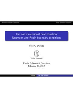
3 The only way heat will leave D is through the boundary . That is, Z. dH. = u n dS. dt D. where D is the boundary of D, n is the outward unit normal vector to D and dS is the surface measure over D. Therefore, we have Z Z. c ut (x, t) dx = u n dS. D D. Recall that for a vector field F , the Divergence Theorem says Z Z. F n dS = F dx. D D. (Ref: See Strauss, Appendix ) Therefore, we have Z Z. c ut (x, t) dx = ( u) dx. D D. This leads us to the partial differential Equation c ut = ( u). If c, and are constants, we are led to the heat Equation ut = k u, Pn where k = /c > 0 and u = i=1 uxi xi . heat Equation on an Interval in R. Separation of Variables Consider the initial/ boundary value problem on an interval I in R.

4 Ut = kuxx x I, t > 0. u(x, 0) = (x) x I ( ).. u satisfies certain BCs. In practice, the most common boundary conditions are the following: 2. 1. Dirichlet (I = (0, l)) : u(0, t) = 0 = u(l, t). 2. Neumann (I = (0, l)) : ux (0, t) = 0 = ux (l, t). 3. Robin (I = (0, l)) : ux (0, t) a0 u(0, t) = 0 and ux (l, t) + al u(l, t) = 0. 4. Periodic (I = ( l, l)): u( l, t) = u(l, t) and ux ( l, t) = ux (l, t). We will give specific examples below where we consider some of these boundary condi- tions. First, however, we present the technique of separation of variables. This technique involves looking for a solution of a particular form. In particular, we look for a solution of the form u(x, t) = X(x)T (t).

5 For functions X, T to be determined. Suppose we can find a solution of ( ) of this form. Plugging a function u = XT into the heat Equation , we arrive at the Equation XT 0 kX 00 T = 0. Dividing this Equation by kXT , we have T0 X 00. = = . kT X. for some constant . Therefore, if there exists a solution u(x, t) = X(x)T (t) of the heat Equation , then T and X must satisfy the equations T0. = . kT. X 00. = . X. for some constant . In addition, in order for u to satisfy our boundary conditions , we need our function X to satisfy our boundary conditions . That is, we need to find functions X. and scalars such that (. X 00 (x) = X(x) x I. ( ). X satisfies our BCs. This problem is known as an eigenvalue problem.)

6 In particular, a constant which satisfies ( ) for some function X, not identically zero, is called an eigenvalue of x2 for the given boundary conditions . The function X is called an eigenfunction with associated eigenvalue . Therefore, in order to find a solution of ( ) of the form u(x, t) = X(x)T (t) our first goal is to find all solutions of our eigenvalue problem ( ). Let's look at some examples below. Example 1. (Dirichlet boundary conditions ) Find all solutions to the eigenvalue problem . X 00 = X 0<x<l ( ). X(0) = 0 = X(l). 3. Any positive eigenvalues? First, we check if we have any positive eigenvalues. That is, we check if there exists any = 2 > 0. Our eigenvalue problem ( ) becomes 00.

7 X + 2X = 0 0<x<l X(0) = 0 = X(l). The solutions of this ODE are given by X(x) = C cos( x) + D sin( x). The boundary condition X(0) = 0 = C = 0. The boundary condition n . X(l) = 0 = sin( l) = 0 = = n = 1, 2, .. l Therefore, we have a sequence of positive eigenvalues n 2. n =. l with corresponding eigenfunctions n . Xn (x) = Dn sin x . l Is zero an eigenvalue? Next, we look to see if zero is an eigenvalue. If zero is an eigenvalue, our eigenvalue problem ( ) becomes 00. X =0 0<x<l X(0) = 0 = X(l). The general solution of the ODE is given by X(x) = C + Dx. The boundary condition X(0) = 0 = C = 0. The boundary condition X(l) = 0 = D = 0. Therefore, the only solution of the eigenvalue problem for = 0 is X(x) = 0.

8 By definition, the zero function is not an eigenfunction. Therefore, = 0 is not an eigenvalue. Any negative eigenvalues? Last, we check for negative eigenvalues. That is, we look for an eigenvalue = 2 . In this case, our eigenvalue problem ( ) becomes 00. X 2X = 0 0<x<l X(0) = 0 = X(l). 4. The solutions of this ODE are given by X(x) = C cosh( x) + D sinh( x). The boundary condition X(0) = 0 = C = 0. The boundary condition X(l) = 0 = D = 0. Therefore, there are no negative eigenvalues. Consequently, all the solutions of ( ) are given by n 2 n . n = Xn (x) = Dn sin x n = 1, 2, .. l l . Example 2. (Periodic boundary conditions ) Find all solutions to the eigenvalue problem . X 00 = X l < x < l ( ).

9 X( l) = X(l), X 0 ( l) = X 0 (l). Any positive eigenvalues? First, we check if we have any positive eigenvalues. That is, we check if there exists any = 2 > 0. Our eigenvalue problem ( ) becomes 00. X + 2X = 0 l < x < l 0 0. X( l) = X(l), X ( l) = X (l). The solutions of this ODE are given by X(x) = C cos( x) + D sin( x). The boundary condition n . X( l) = X(l) = D sin( l) = 0 = D = 0 or = . l The boundary condition n . X 0 ( l) = X 0 (l) = C sin( l) = 0 = C = 0 or = . l Therefore, we have a sequence of positive eigenvalues n 2. n =. l with corresponding eigenfunctions n n . Xn (x) = Cn cos x + Dn sin x . l l 5. Is zero an eigenvalue? Next, we look to see if zero is an eigenvalue. If zero is an eigenvalue, our eigenvalue problem ( ) becomes 00.

10 X =0 l < x < l X( l) = X(l), X 0 ( l) = X 0 (l). The general solution of the ODE is given by X(x) = C + Dx. The boundary condition X( l) = X(l) = D = 0. The boundary condition X 0 ( l) = X 0 (l) is automatically satisfied if D = 0. Therefore, = 0 is an eigenvalue with corresponding eigenfunction X0 (x) = C0 . Any negative eigenvalues? Last, we check for negative eigenvalues. That is, we look for an eigenvalue = 2 . In this case, our eigenvalue problem ( ) becomes 00. X 2X = 0 l < x < l X( l) = X(l), X 0 ( l) = X 0 (l). The solutions of this ODE are given by X(x) = C cosh( x) + D sinh( x). The boundary condition X( l) = X(l) = D sinh( l) = 0 = D = 0. The boundary condition X 0 ( l) = X 0 (l) = C sinh( l) = 0 = C = 0.