Transcription of Chapter 9 Random Numbers - MathWorks
1 Chapter 9. Random Numbers This Chapter describes algorithms for the generation of pseudorandom Numbers with both uniform and normal distributions. Pseudorandom Numbers Here is an interesting number: This is the rst number produced by the Matlab Random number generator with its default settings. Start up a fresh Matlab, set format long, type rand, and it's the number you get. If all Matlab users, all around the world, all on di erent computers, keep getting this same number, is it really Random ? No, it isn't. Computers are (in principle) deterministic machines and should not exhibit Random behavior. If your computer doesn't access some external device, like a gamma ray counter or a clock, then it must really be computing pseudorandom Numbers . Our favorite de nition was given in 1951 by Berkeley professor D.
2 H. Lehmer, a pioneer in computing and, especially, computational number theory: A Random sequence is a vague notion .. in which each term is unpre- dictable to the uninitiated and whose digits pass a certain number of tests traditional with statisticians .. Uniform Distribution Lehmer also invented the multiplicative congruential algorithm, which is the basis for many of the Random number generators in use today. Lehmer's generators involve three integer parameters, a, c, and m, and an initial value, x0 , called the seed. A. September 16, 2013. 1. 2 Chapter 9. Random Numbers sequence of integers is de ned by xk+1 = axk + c mod m. The operation mod m means take the remainder after division by m. For example, with a = 13, c = 0, m = 31, and x0 = 1, the sequence begins with 1, 13, 14, 27, 10, 6, 16, 22, 7, 29, 5, 3.
3 What's the next value? Well, it looks pretty unpredictable, but you've been ini- tiated. So you can compute (13 3) mod 31, which is 8. The rst 30 terms in the sequence are a permutation of the integers from 1 to 30 and then the sequence repeats itself. It has a period equal to m 1. If a pseudorandom integer sequence with values between 0 and m is scaled by dividing by m, the result is oating-point Numbers uniformly distributed in the interval [0, 1]. Our simple example begins with , , , , , , , .. There is only a nite number of values, 30 in this case. The smallest value is 1/31;. the largest is 30/31. Each one is equally probable in a long run of the sequence. In the 1960s, the Scienti c Subroutine Package (SSP) on IBM mainframe computers included a Random number generator named RND or RANDU. It was a multiplicative congruential with parameters a = 65539, c = 0, and m = 231.
4 With a 32-bit integer word size, arithmetic mod 231 can be done quickly. Furthermore, because a = 216 +3, the multiplication by a can be done with a shift and an addition. Such considerations were important on the computers of that era, but they gave the resulting sequence a very undesirable property. The following relations are all taken mod 231 : xk+2 = (216 + 3)xk+1 = (216 + 3)2 xk = (232 + 6 216 + 9)xk = [6 (216 + 3) 9]xk . Hence xk+2 = 6xk+1 9xk for all k. As a result, there is an extremely high correlation among three successive Random integers of the sequence generated by RANDU. We have implemented this defective generator in an M- le randssp. A demon- stration program randgui tries to compute by generating Random points in a cube and counting the fraction that actually lie within the inscribed sphere.
5 With these M- les on your path, the statement will show the consequences of the correlation of three successive terms. The resulting pattern is far from Random , but it can still be used to compute from the ratio of the volumes of the cube and sphere. Uniform Distribution 3. For many years, the Matlab uniform Random number function, rand, was also a multiplicative congruential generator. The parameters were a = 75 = 16807, c = 0, m = 231 1 = 2147483647. These values are recommended in a 1988 paper by Park and Miller [11]. This old Matlab multiplicative congruential generator is available in the M- le randmcg. The statement shows that the points do not su er the correlation of the SSP generator. They generate a much better Random cloud within the cube. Like our toy generator, randmcg and the old version of the Matlab function rand generate all real Numbers of the form k/m for k = 1.
6 , m 1. The smallest and largest are and The sequence repeats itself after m 1 values, which is a little over 2 billion Numbers . A few years ago, that was regarded as plenty. But today, an 800 MHz Pentium laptop can exhaust the period in less than half an hour. Of course, to do anything useful with 2 billion Numbers takes more time, but we would still like to have a longer period. In 1995, version 5 of Matlab introduced a completely di erent kind of Random number generator. The algorithm is based on work of George Marsaglia, a professor at Florida State University and author of the classic analysis of Random number generators, Random Numbers fall mainly in the planes [6]. Marsaglia's generator [9] does not use Lehmer's congruential algorithm. In fact, there are no multiplications or divisions at all. It is speci cally designed to produce oating-point values.
7 The results are not just scaled integers. In place of a single seed, the new generator has 35 words of internal memory or state. Thirty-two of these words form a cache of oating-point Numbers , z, between 0 and 1. The remaining three words contain an integer index i, which varies between 0 and 31, a single Random integer j, and a borrow ag b. This entire state vector is built up a bit at a time during an initialization phase. Di erent values of j yield di erent initial states. The generation of the ith oating-point number in the sequence involves a subtract-with-borrow step, where one number in the cache is replaced with the di erence of two others: zi = zi+20 zi+5 b. The three indices, i, i + 20, and i + 5, are all interpreted mod 32 (by using just their last ve bits). The quantity b is left over from the previous step; it is either zero or a small positive value.
8 If the computed zi is positive, b is set to zero for the next step. But if the computed zi is negative, it is made positive by adding before it is saved and b is set to 2 53 for the next step. The quantity 2 53 , which is half of the Matlab constant eps, is called one ulp because it is one unit in the last place for oating-point Numbers slightly less than 1. 4 Chapter 9. Random Numbers By itself, this generator would be almost completely satisfactory. Marsaglia has shown that it has a huge period almost 21430 values would be generated before it repeated itself. But it has one slight defect. All the Numbers are the results of oating-point additions and subtractions of Numbers in the initial cache, so they are all integer multiples of 2 53 . Consequently, many of the oating-point Numbers in the interval [0, 1] are not represented.
9 The oating-point Numbers between 1/2 and 1 are equally spaced with a spacing of one ulp, and our subtract-with-borrow generator will eventually generate all of them. But Numbers less than 1/2 are more closely spaced and the generator would miss most of them. It would generate only half of the possible Numbers in the interval [1/4, 1/2], only a quarter of the Numbers in [1/8, 1/4], and so on. This is where the quantity j in the state vector comes in. It is the result of a separate, independent, Random number generator based on bitwise logical operations. The oating-point fraction of each zi is XORed with j to produce the result returned by the generator. This breaks up the even spacing of the Numbers less than 1/2. It is now theoretically possible to generate all the oating-point Numbers between 2 53. and 1 2 53.
10 We're not sure if they are all actually generated, but we don't know of any that can't be. Figure shows what the new generator is trying to accomplish. For this graph, one ulp is equal to 2 4 instead of 2 53 . 1. 1/2. 1/4. 1/8. 1/16 1/8 1/4 1/2. Figure Uniform distribution of floating-point Numbers . The graph depicts the relative frequency of each of the oating-point Numbers . A total of 32 oating-point Numbers are shown. Eight of them are between 1/2 and 1, and they are all equally like to occur. There are also eight Numbers between 1/4 and 1/2, but, because this interval is only half as wide, each of them should occur only half as often. As we move to the left, each subinterval is half as wide as the previous one, but it still contains the same number of oating-point Numbers , so their relative frequencies must be cut in half.