Transcription of Conducting a Path Analysis With SPSS/AMOS
1 Conducting a path Analysis with SPSS/AMOS . Download the data file from my spss data page and then bring it into spss . The data are those from the research that led to this publication: Ingram, K. L., Cope, J. G., Harju, B. L., & Wuensch, K. L. (2000). Applying to graduate school: A test of the theory of planned behavior. Journal of Social Behavior and Personality, 15, 215-226. Obtain the simple correlations among the variables: Attitude SubNorm PBC Intent Behavior Attitude .472 .665 .767 .525. SubNorm .472 .505 .411 .379. PBC .665 .505 .458 .496. Intent .767 .411 .458 .503. Behavior .525 .379 .496 .503 One can conduct a path Analysis with a series of multiple regression analyses. We shall test a model corresponding to Ajzen's Theory of Planned Behavior look at the model presented in the article cited above, which is available online.
2 Notice that the final variable, Behavior, has paths to it only from Intention and PBC. To find the coefficients for those paths we simply conduct a multiple regression to predict Behavior from Intention and PBC. Here is the output. Model Summary Adjusted R Std. Error of the Model R R Square Square Estimate a 1 .585 .343 .319 a. Predictors: (Constant), PBC, Intent b ANOVA. Model Sum of Squares df Mean Square F Sig. a 1 regression 2 .000. Residual 57 Total 59. a. Predictors: (Constant), PBC, Intent b. Dependent Variable: Behavior Beta t Sig. (Constant) .281. Intent .350 .005. PBC .336 .007. The Beta weights are the path coefficients leading to Behavior: .336 from PBC and .350 from Intention. 2. In the model, Intention has paths to it from Attitude, Subjective Norm, and Perceived Behavioral Control, so we predict Intention from Attitude, Subjective Norm, and Perceived Behavioral Control.
3 Here is the output: Model Summary Adjusted R Std. Error of the Model R R Square Square Estimate a 1 .774 .600 .578 a. Predictors: (Constant), PBC, SubNorm, Attitude b ANOVA. Model Sum of Squares df Mean Square F Sig. a 1 regression 3 .000. Residual 56 Total 59. a. Predictors: (Constant), PBC, SubNorm, Attitude b. Dependent Variable: Intent Beta t Sig. (Constant) .037. Attitude .807 .000. SubNorm .095 .946 .348. PBC .290. The path coefficients leading to Intention are: .807 from Attitude, .095 from Subjective Norms, and .126 from Perceived Behavioral Control. amos . Since students at ECU no longer have access to amos , I am not going to cover it this semester. Now let us use amos . The data file is already open in spss . Click Analyze, IBM spss . amos .
4 In the amos window which will open click File, New: 3. You are going to draw a path diagram like that on the next page. Click on the Draw observed variables icon which I have circled on the image above. Move the cursor over into the drawing space on the right. Keep your drawing in the central, white, area not let it extend into the gray area bounding it. Hold down the left mouse button while you move the cursor to draw a rectangle. Release the mouse button and move the cursor to another location and draw another rectangle. Annoyed that you can't draw five rectangles of the same dimensions. Do it this way instead: Draw one rectangle. Now click the Duplicate Objects icon, boxed in black in the image to the right, point at that rectangle, hold down the left mouse button while you move to the desired location for the second rectangle, and release the mouse button.
5 You can change the shape of the rectangles later, using the Change the shape of objects tool (boxed in green in the image to the right), and you can move the rectangles later using the Move objects tool (boxed in blue in the image to the right). Click on the List variables in data set icon (boxed in orange in the image to the right). From the window that results, drag and drop variable names to the boxes. A more cumbersome way to do this is: Right-click the rectangle, select Object Properties, then enter in the Object Properties window the name of the observed variable. Close the widow and enter variable names in the remaining rectangles in the same way. Click on the Draw paths icon (the single-headed arrow boxed in purple in the image above) and then draw a path from Attitude to Intent (hold down the left mouse button at the point you wish to start the path and then drag it to the ending point and release the mouse button).
6 Also draw paths from SubNorm to Intent, PBC to Intent, PBC to Behavior, and Intent to Behavior. Click on the Draw Covariances icon (the double-headed arrow boxed in purple in the image above) and draw a covariance from SubNorm to Attitude. Draw another from PBC. to SubNorm and one from PBC to Attitude. You can use the Change the shape of objects tool (boxed in green in the image above) to increase or decrease the arc of these covariances just select that tool, put the cursor on the path to be changed, hold down the left mouse button, and move the mouse. 4. Click on the Add a unique variable to an existing variable icon (boxed in red in the image above) and then move the cursor over the Intent variable and click the left mouse button to add the error variable.
7 Do the same to add an error variable to the Behavior variable. Right-click the error circle leading to Intent, select Object Properties, and name the variable e1. Name the other error circle e2.. Click the Analysis properties icon -- to display the Analysis Properties window. On the Estimation and Output tabs check boxes as shown below. 5. Indirect effects are best tested with bootstrapping methods. Click the bootstrap tab and check the boxes as indicated to the right. Ask for 2,000 bootstrap samples and 95%. confidence. Click on the Calculate estimates icon . In the Save As window browse to the desired folder and give the file a name. Click Save. Click the View the output path diagram setting (boxed in red in the image to the right). You will get the path diagram with unstandardized coefficients.
8 Click the Copy the path diagram to the clipboard icon. Open a Word document or photo editor and paste in the path diagram. 6. The coefficients here are unstandardized that is, covariances and slopes. If you want standardized coefficients (correlation coefficients and beta weights), click Standardized estimates in the pane shown to the right Click the View text icon to see extensive text output from the Analysis . 7. The Copy to Clipboard icon (green dot, above) can be used to copy the output to another document via the clipboard. Click the Options icon (red dot, above) to select whether you want to view/copy just part of the output or all of the output. Here are some parts of the output with my comments: Variable Summary (Group number 1). Your model contains the following variables (Group number 1).
9 Observed, endogenous variables Intent Behavior Observed, exogenous variables Attitude PBC. SubNorm Unobserved, exogenous variables e1. e2. Variable counts (Group number 1). Number of variables in your model: 7. Number of observed variables: 5. Number of unobserved variables: 2. Number of exogenous variables: 5. Number of endogenous variables: 2. 8. Parameter summary (Group number 1). Weights Covariances Variances Means Intercepts Total Fixed 2 0 0 0 0 2. Labeled 0 0 0 0 0 0. Unlabeled 5 3 5 0 0 13. Total 7 3 5 0 0 15. Models Default model (Default model). Notes for Model (Default model). Computation of degrees of freedom (Default model). Number of distinct sample moments: 15. Number of distinct parameters to be estimated: 13. Degrees of freedom (15 - 13): 2.
10 Result (Default model). Minimum was achieved Chi-square = .847. Degrees of freedom = 2. Probability level = .655. This Chi-square tests the null hypothesis that the overidentified (reduced) model fits the data as well as does a just-identified (full, saturated) model. In a just-identified model there is a direct path (not through an intervening variable) from each variable to each other variable. In such a model the Chi-square will always have a value of zero, since the fit will always be perfect. When you delete one or more of the paths you obtain an overidentified model and the value of the Chi-square will rise (unless the path (s) deleted have coefficients of exactly zero). For any model, elimination of any (nonzero) path will reduce the fit of model to data, increasing the value of this Chi-square, but if the fit is reduced by only a small amount, you will have a better model in the sense of it being less complex and explaining the covariances almost as well as the more complex model.