Conduction Heat transfer: Unsteady state - CHERIC

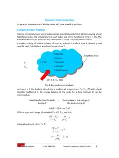
1 Conduction heat transfer: Unsteady stateChapter ObjectivesFor solving the situations that Where temperatures do not change with position. In a simple slab geometry where temperature vary also with position. Near the surface of a large body (semi infinite region)Keywords Internal resistance External resistance Biot number Lumped parameter anaysis 1D and multi dimensional heat Conduction Heisler charts Semi infinite region1 Lumped Parameter AnalysisIn transient, Tr=rTr=0Tr= 1. Several temperatures in the Parameter AnalysisFigure 2. A solid with convection over its surface.) tThA(T TmCp (1)) ThA(T TmCp M : MassCp: Specific heath : Convective heat transfer coefficientA : Surface areaT : Bulk fluid temperature(1)(2)Lumped Parameter Analysis(3)Lumped Parameter Analysis(5)(4)2 Biot NumberTr=rTr= 3. Several temperatures in the , when can we apply ?Biot NumberBi (Biot Number) : Deciding whether internal resistance can be ignored.

2 (6)(7)Characteristic LengthCharacteristic length V/APath of least thermal resistanceCharacteris c length = Temperature can be changedin short timeFigure 4. Characteristic lengths for heat Conduction in various geometries.(8)What is the temperature of the egg after 60min?Figure 5. Schematic for Example 1 Known: Initial temperature of an eggFind: Temperature of the egg after data: T i= 20 CT air=38 Ch = W/m2 K = 1035 kg/m3Cp= 3350 J/kg Kk = W/m KBeing Bi < , lumped analysis can be applied!Assumption: 1. Egg is approximately Surface heat transfer coefficient provided is an average Lumped parameter (Biot Number) = hV / Ak = < (Eqn. 5),Then, T = CBeing Bi < , lumped analysis can be applied!Assumption: 1. Egg is approximately Surface heat transfer coefficient provided is an average Lumped parameter (Biot Number) = hV / Ak = < ( ),Then, T = C3 When Internal Resistance Is Not NegligibleTr=rTr= 1: Several temperatures in the situations,Tr=rTr=0Tr= ( Bi )When Internal Resistance Is Not NegligibleFigure 6.

3 Schematic of a slab showing the line of symmetry at x = 0 and the two surfcaes at x = L and at x = L maintained at temperature TS. The material is very large (extends to infinity) in the other two Internal Resistance Is Not Negligible(9)(10)(11)Boundary conditionsWhen Internal Resistance Is Not Negligible(12)Initial condition(13) (Thermal diffusivity) = k/ CpHow Temperature Changes with TimeFigure 7. The terms in the series (n = 0, 1, .. in Equation ) drop off rapidly for values of time. Calculations are for FO= at 30 s and FO= at 600 s for a thickness of L = m and a typical = x 10 7m2/s for bio visualizing Temperature vs. Position and Time,infinite series should be simplifiedHow Temperature Changes with TimeComparingdifferent termsat each time(t= 30s, t= 600s),Contribution decaysGradually at t= 30sRapidly at t= 600s (15)(16)Temperature Change with Position and Spatial Average We can see that temperature varies as a cosine function Therefore, we need to define spatial average temperature(15)(16)tLsiseLxTTTT222cos4 tLLxTTTTsis222cos4lnln Spatial average temperature(17)(18)Applying ( ) to ( ) gives LavTdxLT01tLTTTT sisav2228lnln Temperature Change with Size(19) sisavTTTTLt8ln4222 Charts Developed from the Solutions: Their Uses and Limitations.

4 It can be seen that temperature is a function of x/L and t/L2 Charts are developed because of the complexity of the calculation of series.(20) 222120212cos1214 LtnnnsiseLxnnTTTT Charts are developed with the condition of n=0. In other words, it is a plot of Eqn. 5 And it is also called Heisler chart. There are some assumptions for the development of the charts. These are:1. Uniform initial temperature2. Constant boundary fluid temperature3. Perfect slab, cylinder or sphere4. Far from edges5. No heat generation (Q=0)6. Constant thermal properties (k, , cpare constants)7. Typically for times long after initial times, given by t/L2> 8. Unsteady state diffusion in a large slabExample 2. Temperatures Reached During Food Sterilization Surface temperature of a slab of tuna is suddenly increased Find the temperature at the center of the slab after 30 minFigure 9.

5 A cylindrical can containing food to be sterilized. Given data:1. Thickness of slab = 25 mm2. Thermal diffusivity of the slab,3. Initial temperature = 40 C4. Surface temperature = 121 C5. Time of heating = 1800s Assumptions1. Heating from the side is ignored2. Thermal diffusivity is constantsm/10227 So the temperature T = C after 30 minutes of Lxn0 hLkm mssmLtF TTTTiConvective Boundary Condition We have considered a negligible external fluid resistance to heat transfer. But if we consider external fluid resistance in addition to internal fluid resistance,Figure 10. In convective boundary condition, surface temperature is not the same as the bulk fluid temperature, T , signifying additional fluid resistance. At the surface,The solution is generalized form of Eqn. and you can refer to Heisler chart as well. TThxTkssNumerical Methods as Alternatives to the Charts In practice, however, such conditions dealt with above are not that simple Limitations of the analytical solutions can be overcome using numerical, computer based solutions4 Transient heat Transfer in a Finite Geometry Multi Dimensional Problems We should consider the situation two and three dimensional effect yields A finite geometry is considered as the intersection of two or three infinite geometries(21)slabzinitesistzslabyinites istyslabxinitesistxsistxyzTTTTTTTTTTTTTT TTinf,inf,inf,, Figure 11.

6 A finite cylinder can be considered as an intersection of an infinite cylinder and a slabslabinitesistzcylinderinitesistrsist zrTTTTTTTTTTTTinf,inf,,, (22)5 Transient heat Transfer in a Semi infinite Region A semi infinite region extends to infinity in two directions and a single identifiable surface in the other direction You can see Fig. extends to infinity in the y and z directions and has an identifiable surface at x=0 Figure 12. Schematic of a semi-infinite region showing only one identifiable surface. It can be used practically in heat transfer for a relatively short time and/or in a relatively thick material The governing equation with no bulk flow and no heat generation is The boundary conditions are The initial condition is22xTtT sTxT 0 iTxT iTtT 0(23)(24)(25)(26) The solution is txerfTTTTisi 21(27)The function erf( ) is called error function and given bytx 2 022)(deerfAnd here,Figure 13.

7 Comparison of the complementary error function (1-erf( )) with an exponential e- heat flux at the surface of the semi infinite region can be calculated with chain rule00" xxsdxdddTkdxdTkq tTTkteTTkisis 21202(28) The situation we can approximate semi infinite regionFigure 14. Plot of Eqn. 29, illustrating the minimum thickness of a material for which error function solution can be 422 (29) Other boundary conditions1. Convective boundary condition TThxTksurfacesurfaceThe solution is kthtxerfetxerfTTTT kthkhxii 212122(30)2. Specified surface heat flux boundary condition""ssurfaceqq (31) txerfkxqetqkTTstxsi 212"4"2(32)The solution isExample 3 Analysis of Skin BurnsFigure 15. Section of a skin with degrees of burn superimposed on it. A thermal burn occurs as a result of an elevation in tissue temperature above a threshold value for a finite period of time The intensity of thermal burn is divided into four degrees6 Chapter Summary Transient heat Conduction No Internal Resistance, Lumped Parameter1.

8 The thermal resistance of the solid can be ignored if a Biot number is less than As thermal resistances are ignored, temperature is a function of time only. Internal Resistance is Significant1. When internal resistance is significant (Bi> ), temperature is a function of both position and time2. For an infinite slab, infinite cylinder and spherical geometry, the solutions are given as Heisler chart. You can find it on pages 327~ For finite slab and finite cylinder, the solutions are intersection of the infinite slabs and Materials with thickness are considered effectively semi infinitetL 4