Conduction in the Cylindrical Geometry - Clarkson University

1 1 Conduction in the Cylindrical Geometry R. Shankar Subramanian Department of Chemical and Biomolecular Engineering Clarkson University Chemical engineers encounter Conduction in the Cylindrical Geometry when they analyze heat loss through pipe walls, heat transfer in double-pipe or shell-and-tube heat exchangers, heat transfer from nuclear fuel rods, and other similar situations. Unlike Conduction in the rectangular Geometry that we have considered so far, the key difference is that the area for heat flow changes from one radial location to another in the Cylindrical Geometry .

2 This affects the temperature profile in steady Conduction . As an example, recall that the steady temperature profile for one-dimensional Conduction in a rectangular slab is a straight line, provided the thermal conductivity is a constant. In the Cylindrical Geometry , we find the steady temperature profile to be logarithmic in the radial coordinate in an analogous situation. To see why, let us construct a model of steady Conduction in the radial direction through a Cylindrical pipe wall when the inner and outer surfaces are maintained at two different temperatures.

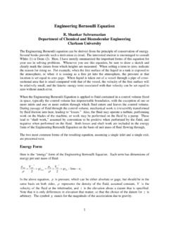
3 Steady Conduction Through a Straight Cylindrical Pipe Wall Consider a straight circular pipe of inner radius 1r, outer radius 2r and length L depicted below. Let the steady temperature of the inner surface be 1T and that of the outer surface be 2T, as shown on the sketch. The temperature varies only in the radial direction. For modeling heat flow through the pipe wall, it is convenient to use the end view shown on the following page. zr1r2r2T1TL2 We use a shell balance approach. Consider a Cylindrical shell of inner radius r and outer radius rr+ located within the pipe wall as shown in the sketch.

4 The shell extends the entire length L of the pipe. Let ( )Qr be the radial heat flow rate at the radial location r within the pipe wall. Then, in the end view shown above, the heat flow rate into the Cylindrical shell is ( )Qr, while the heat flow rate out of the Cylindrical shell is ()Qrr+ . At steady state, ( ) ()Qr Qrr= + . Rearrange this result after division by r as shown below. () ( )0 Qrr Qrr+ = Now take the limit as 0r . This leads to the simple differential equation 0dQdr= Integration is straightforward, and leads to the result constantQ= independent of radial location.

5 The heat flow rate rQ qA=, where A is the area of the Cylindrical surface normal to the r direction, and rq is the heat flux in the radial direction. The area of the Cylindrical surface is 2 ArL =, where L is the length of the pipe. From Fourier s law, rdTqkdr= . Therefore, we find that 1r2r1T2 Trr ( )Qr()Qrr+ 3 constantdTAkdr = Substituting for the area A, we can write 2constantdTrLkdr =. Because 2Lk is constant, this leads to a simple differential equation for the temperature distribution in the pipe wall.

6 1dTrCdr= Here, 1C is a constant that needs to be determined later. Rearrange this equation as 1drdTCr= and integrate both sides to yield 12lnTC r C=+ where 2C is another constant that needs to be determined. Thus, we find that the steady state temperature distribution in the pipe wall for constant thermal conductivity is logarithmic, in contrast to Conduction through a rectangular slab in which case, the steady temperature distribution was found to be linear. To find the two constants in the solution, we must use boundary conditions on the temperature distribution.

7 The temperature is specified at both the inner and outer pipe wall surfaces. Thus, we can write the boundary conditions as follows. ( )11Tr T= ()22Tr T= By substituting these two boundary conditions in the solution for the temperature field in turn, we obtain two equations for the undetermined constants 1C and 2C. 1 11 2lnTC r C=+ 2 12 2lnTC r C=+ These two linear equations can be solved for the values of the constants 1C and 2C in a straightforward manner. We find ()12112ln/TTCrr = ()1221112lnln/TTCTrrr = Substituting the results for the two constants in the solution for the temperature profile, followed by rearrangement, yields the following result for the temperature distribution in the pipe wall.

8 ( )()111 221ln/ln/rrTTT Trr = 4 A sample sketch of the steady temperature profile in the pipe wall is shown below. We are ready to evaluate the heat flow rate Q. 2rdTQq AkrLdr = = Recall that 1//dT drC r=. Substituting in the result for Q leads to ()()()121211221222ln/ln/TTTTQkCLLkLkrrr r = = = This result is a bit hard to remember. Let us try recasting it in a form similar to that we used for steady Conduction in a rectangular slab. Let us write TQR = where 12 TTT = is the driving force, and R is the resistance to heat flow.

9 We find that the resistance is () ()21ln// 2Rr rLk =. Let us rearrange this result. 1T2T1r2r5 ()()[]()2121212121212121ln/ln/2222ln 2/ 2lmrrrrrrrrrrRLkrrLkkAkLrLrLrLr == == where we have introduced a new symbol lmA, which stands for log mean area. It is defined as ()2121ln/lmAAAAA = where 112 ALr = is the inner surface area of the pipe wall, and 222 ALr = is the outer surface area of the pipe wall. The log mean always lies between the two values being averaged. Try comparing it with the more common arithmetic average, which is 122AA+.

10 You will find that the log mean is always smaller than the arithmetic average. For ()21/2AA , the difference between the two averages is less than 4%. Steady Conduction Through Multiple Layers in the Cylindrical Geometry It is straightforward to extend our analysis of steady state Conduction in a pipe wall to multiple layers in the Cylindrical Geometry . Consider, for example, a pipe of length L carrying hot or cold fluid that needs to be insulated from the surroundings. We add an insulation layer to the outside of the pipe.