Transcription of Creating a Gradebook in Excel - University of California, San …
1 Creating a Spreadsheet Gradebook1 Creating a Gradebook in ExcelSpreadsheets are a great tool for Creating gradebooks. With a little bit of work,you can create a customized Gradebook that will provide weighted scores and following instructions describe the steps for Creating a spreadsheet LayoutLet s start by laying out Gradebook (see Figure 1).Figure 1 Gradebook LayoutFirst, we created a title, First Term Fall 2001, so that we could identify the , we added labels for the various columns. Columns A & B are for student sample Gradebook is simple in that it only has homework assignments and tests.
2 Wehave created column groupings ( , Homework Assignments and Tests) and columnheadings ( , Week 1, Week 2, etc) for our assessments. For this class we will averageall the scores and compute the final FormulasOur next step is to create a formula to calculate average. The following steps are forExcel. Other spreadsheets use a similar procedure, but may use a different Start by clicking in the cell where you want the average to appear. We selectedcell I5 (see Figure 1) which is the average for our first Select Function from the Insert menu.
3 Excel will display the Paste Functiondialog (see Figure 2). Select Statistical from the left list and Average from theright list. Then, click Ok. (Sometimes the Average function will appear when youclick on the Most Recently Used category.) Creating a Spreadsheet Gradebook2 Figure 2 Paste Function Dialog3. When you see the Average dialog displayed (Figure 3), click the red arrow to theright of Number 3 Average DialogCreating a Spreadsheet Gradebook34. The dialog box is hidden and you can select the cells to include in the the cursor to select all the cells that will have scores or grades in row 5 (seeFigure 4).
4 Notice how the range of cells is displayed in the text entry box and incell Once you have selected the cells, click the red icon to the right of the area listingthe cells in the formula. Then, click Ok when the Average dialog box you have entered data into the cells, the average will appear in the We could repeat these steps for each student, but there is an easier way toduplicate the formula for each student. Our Gradebook will have five students, sowe selected cells I5 through I9 by dragging our cursor.
5 Next, we selected Fillfrom the Edit menu, then Down from the Fill menu (see Figure 5). When wereleased the cursor, Excel created a formula in each cell. (Shortcut: aftercomputing the Average in cell I5, click on cell I5, place your cursor over thesquare in the bottom right of the cell, and drag the square to cell I9. Excel will beautomatically create the Average formula in each cell.)Figure 5 Filling in cells7. Now, we can add our students and some data to the cells. Figure 6 shows ourcompleted 4 Selecting Cells for a FormulaClick to FinishCreating a Spreadsheet Gradebook4 Figure 6 Completed Gradebook8.
6 We need to make another fix with our Gradebook . Notice that the averages aredisplayed with 5 decimal points. We could select any number, but for thisgradebook, we want whole numbers. To change the formatting of the numbers,select the cells and then select Cells from the Format menu. When the Formatdialog is displayed select Numbers from the list and then select 0 as the number ofdecimal positions to display (See Figure 7).Figure 7 Format Cells Dialog9. Now, our spreadsheet is nice and neat, but we need to convert the average scoresto a letter grade for the report card.
7 Entering the grades for just five students thetask is not a big chore, however, a class of 30 students or 5 classes of 30 studentscan take a lot of time to assign letter grades. We can add one more function tolookup the We need to start by first Creating a grading scale (see Figure 8). Create this tablein any blank area of your spreadsheet. You can also include A-, B+, etc. Just keepeverything in order from low to a Spreadsheet Gradebook5 Figure 8 Table with Grading Scale11. Select the cell for the first student s letter grade (J5 in our example).
8 We willcreate a formula to lookup the student s letter grade based on the Average. Theformula uses the format =LOOKUP (Average grade Cell, Range of the table, thecolumn for the letter grade ). The student s average grade is in cell I5. Our gradelookup table is spread over two columns and we define it by listing the top leftcell and the bottom right cell (B14 and C18). We will look the grade up in thesecond column of the does it work? Let s use the first average of 82 as an example. Excel goes toour table and compares 82 to the values in the first column.
9 It searches until itfinds a value higher than 82. When it compares 82 to the table of value of 89, itstops and uses the previous cell as 82 is between 79 and 89. Excel then looks intothe second column and selects the contents, which is B to put in our gradecolumn. If the student had an average of 95, then Excel would choose the lettergrade from the highest Let s create the LOOKUP formula. First click on cell J5. Next, type the followinginto the text entry box=LOOKUP (I5,$B$14:$C$18,2)We put dollar signs around the cell referents so that Excel would use them todefine our lookup table.
10 Our formula tells Excel to take the average score fromCell I5, find it s location in our table consisting of two columns spanning fromB14 to C18, and then use the letter grade in the second Press return after you enter your formula and the grade should appear. You cannow use the Fill function to create a formula for each remaining student (seeFigure 9). (Shortcut: after Creating the formula in cell J5, select cell J5, place yourcursor over the square in the cell s bottom right corner, and drag to cell J9. TheLOOKUP formula is automatically created in each cell.)