Transcription of Creating and Customizing the Kaplan-Meier …
1 Paper SP14 SAS-2014 Creating and Customizing the Kaplan-Meier survival Plot in PROCLIFETEST in the SAS/STAT ReleaseWarren F. Kuhfeld and Ying So, SAS Institute you are a medical, pharmaceutical, or life sciences researcher, you have probably analyzed time-to-eventdata ( survival data). The LIFETEST procedure computes Kaplan-Meier estimates of the survivor functionsand compares survival curves between groups of patients. You can use the Kaplan-Meier plot to display thenumber of subjects at risk, confidence limits, equal-precision bands, Hall-Wellner bands, and homogeneitytestp-value. You can control the contents of the survival plot by specifying procedure options in PROCLIFETEST.
2 When the procedure options are insufficient, you can modify the graph templates by using SASmacros. PROC LIFETEST in SAS/STAT provides many new options for Kaplan-Meier plot modification,and the macros have been completely redone in this release in order to provide more power and flexibilitythan was available in previous releases. This paper provides examples of these new that measure lifetime or the length of time until the occurrence of an event are data are often medical data; examples include the survival time for heart transplant or cancerpatients. survival time is a measure of the duration of time until a specified event (such as relapse or death)occurs.
3 survival data consist of survival time and possibly a set of independent variables that are thoughtto be associated with the survival time variable. The system that gives rise to the event of interest can bebiological (as with most medical data) or physical (as with engineering data). survival analysis estimatesthe underlying distribution of the survival time variable and assesses the dependence of the survival timevariable on the independent data analysis methods are not appropriate for survival data. In general, survival times are positivelyskewed, and it is not reasonable to assume that data of this type have a normal distribution. Furthermore, survival times are often censored.
4 The survival time of an individual is right-censored when the event ofinterest has not been observed for that individual. For example, a patient who is recruited for a clinical trialdrops out of the trial or the event is not observed when the period of data collection ends. In either case, theobserved time is less than the true survival time. Analysis of survival data must take censoring into accountand correctly use both the censored observations and the uncensored LIFETEST procedure in SAS/STAT is a nonparametric procedure for analyzing survival data. You canuse PROC LIFETEST to compute the Kaplan-Meier (1958) curve, which is a nonparametric maximumlikelihood estimate of the survivor function.
5 You can display the Kaplan-Meier plot, which contains stepfunctions that represent the Kaplan-Meier curves of different samples. You can also use PROC LIFETEST tocompare the survivor functions of different samples by the log-rank data that are used in this paper come from 137 bone marrow transplant patients in a study by Klein andMoeschberger (1997) and are available in the BMT data set in the Sashelp library. At the time of transplant,each patient is classified in one of three risk categories: ALL (acute lymphoblastic leukemia), AML (acutemyelocytic leukemia) Low Risk, and AML High Risk. The endpoint of interest is the disease-free survivaltime, which is the time in days until death, relapse, or the end of the study.
6 The variableGrouprepresentsthe patient s risk category, the variableTrepresents the disease-free survival time, and the variableStatusis the censoring indicator. A status of 1 indicates an event time, and a status of 0 indicates a censored examples use the release of SAS/STAT software from 2013. Three types of examples are provided:specifying procedure options, modifying graph templates, and modifying style THE survival PLOT BY SPECIFYING PROCEDURE OPTIONSYou can use the following statements to enable ODS Graphics and run PROC LIFETEST:ods graphics on;proc lifetest data= ;time T*Status(0);strata Group;run;The results, displayed in Figure 1, consist of three step functions, one for each of the three groups of plot shows that patients in the AML Low Risk group have longer disease-free survival times thanpatients in the ALL and AML High Risk 1 Default Kaplan-Meier PlotYou specify in the TIME statement that the disease-free survival time is recorded in the variableT.
7 You furtherspecify that the variableStatusindicates censoring and 0 indicates a censored time. Separate survivorfunctions are displayed for each group in theGroupvariable, which you specify in the STRATA Graphics is enabled for this step and all subsequent steps until it is disabled. (ODS Graphics remainsenabled throughout the examples in this paper.) The survival plot is produced by default when ODS Graphicsis enabled. You can add the option PLOTS= survival to the PROC LIFETEST statement to explicitly requestthe survival plot, but that is equivalent to the default. Usually, you use the PLOTS= survival optionwhen you want to specify plot-specific options. You can use the PLOTS= option to request nondefault graphsand specify options for some graphs.
8 You can specify graph names (PLOTS= survival ), graph options(PLOTS= survival (ATRISK OUTSIDE)), and suboptions (PLOTS= survival (ATRISK OUTSIDE( ))).You can use the STRATA=INDIVIDUAL option to request individual survival plots. By default, theSTRATA=OVERLAY option produces the plot of overlaid step functions that is displayed in Figure 1. You canrun the same analysis but request the results in three separate graphs, one per patient group, as follows:proc lifetest data= plots= survival (strata=individual);time T*Status(0);strata Group;run;The first of the three survival plots is displayed in Figure 2. To conserve space, the other graphs are 2 One of Three Individual PlotsYou can use the STRATA=PANEL option as follows to display the results in separate panels of a single graph:proc lifetest data= plots= survival (strata=panel);time T*Status(0);strata Group;run;The results are displayed in Figure 3.
9 The rest of this paper discusses overlaid plots such as the onedisplayed in Figure 3 Individual Plots Displayed in a Panel3 You can use the following statements to add Hall-Wellner confidence bands (Hall and Wellner 1980) toFigure 1 and display thep-value from a test that the strata are homogeneous:proc lifetest data= plots= survival (cb=hw test);time T*Status(0);strata Group;run;The results are displayed in Figure 4. The Hall-Wellner confidence bands extend to the last event times. Thesmallp-value supports rejecting the hypothesis that the groups are 4 Confidence Bands and Homogeneity TestYou can use the following statements to add equal-precision bands to the plot:proc lifetest data= plots= survival (cb=ep test);time T*Status(0);strata Group;run;The results are displayed in Figure 5 Equal-Precision BandsYou can use the following statements to add both Hall-Wellner and equal-precision bands to the plot:proc lifetest data= plots= survival (cb=all test);time T*Status(0);strata Group;run.
10 The results are displayed in Figure 6 Hall-Wellner and Equal-Precision Bands5 You can display the patients-at-risk table in the Kaplan-Meier plot as follows:proc lifetest data= plots= survival (cb=hw test atrisk);time T*Status(0);strata Group;run;The results are displayed in Figure 7. By default, the at-risk table is displayed inside the body of the table shows the number of patients in each group who are at risk for each of the different times. Forthese data, the default survival times at which at-risk values are displayed are 0 to 2500 by 500. You will seehow to specify other values in subsequent 7At-Risk Table inside the PlotThe group labels for the at-risk table are group numbers, and these numbers appear in the legend.